Statistical Modeling with a Single Mediator
2024-07-01
Source:vignettes/single_mediator.Rmd
single_mediator.RmdThis example demonstrates how to use cmest when there is
a single mediator. For this purpose, we simulate some data containing a
continuous baseline confounder \(C_1\),
a binary baseline confounder \(C_2\), a
binary exposure \(A\), a binary
mediator \(M\) and a binary outcome
\(Y\). The true regression models for
\(A\), \(M\) and \(Y\) are: \[logit(E(A|C_1,C_2))=0.2+0.5C_1+0.1C_2\]
\[logit(E(M|A,C_1,C_2))=1+2A+1.5C_1+0.8C_2\]
\[logit(E(Y|A,M,C_1,C_2)))=-3-0.4A-1.2M+0.5AM+0.3C_1-0.6C_2\]
## Registered S3 methods overwritten by 'lme4':
##   method                          from
##   cooks.distance.influence.merMod car
##   influence.merMod                car
##   dfbeta.influence.merMod         car
##   dfbetas.influence.merMod        car
set.seed(1)
expit <- function(x) exp(x)/(1+exp(x))
n <- 10000
C1 <- rnorm(n, mean = 1, sd = 0.1)
C2 <- rbinom(n, 1, 0.6)
A <- rbinom(n, 1, expit(0.2 + 0.5*C1 + 0.1*C2))
M <- rbinom(n, 1, expit(1 + 2*A + 1.5*C1 + 0.8*C2))
Y <- rbinom(n, 1, expit(-3 - 0.4*A - 1.2*M + 0.5*A*M + 0.3*C1 - 0.6*C2))
data <- data.frame(A, M, Y, C1, C2)
The DAG for this scientific setting is:
cmdag(outcome = "Y", exposure = "A", mediator = "M",
      basec = c("C1", "C2"), postc = NULL, node = TRUE, text_col = "white")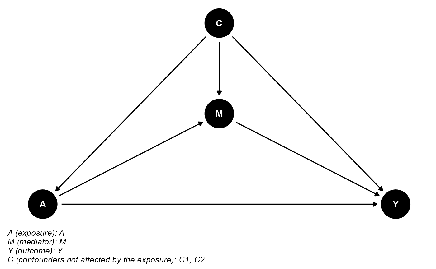
In this setting, we can use all of the six statistical modeling approaches. The results are shown below:
The Regression-based Approach
Closed-form Parameter Function Estimation and Delta Method Inference
res_rb_param_delta <- cmest(data = data, model = "rb", outcome = "Y", exposure = "A",
                            mediator = "M", basec = c("C1", "C2"), EMint = TRUE,
                            mreg = list("logistic"), yreg = "logistic",
                            astar = 0, a = 1, mval = list(1),
                            estimation = "paramfunc", inference = "delta")
summary(res_rb_param_delta)## Causal Mediation Analysis
##
## # Outcome regression:
##
## Call:
## glm(formula = Y ~ A + M + A * M + C1 + C2, family = binomial(),
## data = getCall(x$reg.output$yreg)$data, weights = getCall(x$reg.output$yreg)$weights)
##
## Deviance Residuals:
## Min 1Q Median 3Q Max
## -0.5681 -0.2414 -0.1741 -0.1604 3.0521
##
## Coefficients:
## Estimate Std. Error z value Pr(>|z|)
## (Intercept) -3.5731 0.7713 -4.633 3.61e-06 ***
## A 0.7084 0.5283 1.341 0.17990
## M -1.0471 0.3736 -2.803 0.00507 **
## C1 0.9337 0.6973 1.339 0.18054
## C2 -0.8415 0.1443 -5.829 5.56e-09 ***
## A:M -0.4222 0.5541 -0.762 0.44607
## ---
## Signif. codes: 0 '***' 0.001 '**' 0.01 '*' 0.05 '.' 0.1 ' ' 1
##
## (Dispersion parameter for binomial family taken to be 1)
##
## Null deviance: 2022.7 on 9999 degrees of freedom
## Residual deviance: 1965.0 on 9994 degrees of freedom
## AIC: 1977
##
## Number of Fisher Scoring iterations: 7
##
##
## # Mediator regressions:
##
## Call:
## glm(formula = M ~ A + C1 + C2, family = binomial(), data = getCall(x$reg.output$mreg[[1L]])$data,
## weights = getCall(x$reg.output$mreg[[1L]])$weights)
##
## Deviance Residuals:
## Min 1Q Median 3Q Max
## -3.2578 0.1145 0.1647 0.2519 0.5563
##
## Coefficients:
## Estimate Std. Error z value Pr(>|z|)
## (Intercept) 0.4353 0.6410 0.679 0.49712
## A 1.7076 0.1443 11.837 < 2e-16 ***
## C1 1.9982 0.6474 3.086 0.00203 **
## C2 0.9024 0.1345 6.709 1.96e-11 ***
## ---
## Signif. codes: 0 '***' 0.001 '**' 0.01 '*' 0.05 '.' 0.1 ' ' 1
##
## (Dispersion parameter for binomial family taken to be 1)
##
## Null deviance: 2294.0 on 9999 degrees of freedom
## Residual deviance: 2072.5 on 9996 degrees of freedom
## AIC: 2080.5
##
## Number of Fisher Scoring iterations: 7
##
##
## # Effect decomposition on the odds ratio scale via the regression-based approach
##
## Closed-form parameter function estimation with
## delta method standard errors, confidence intervals and p-values
##
## Estimate Std.error 95% CIL 95% CIU P.val
## Rcde 1.33138 0.22278 0.95912 1.848 0.0872 .
## Rpnde 1.41988 0.23708 1.02358 1.970 0.0358 *
## Rtnde 1.34928 0.22056 0.97940 1.859 0.0669 .
## Rpnie 0.93338 0.03576 0.86587 1.006 0.0719 .
## Rtnie 0.88697 0.05295 0.78902 0.997 0.0445 *
## Rte 1.25939 0.19804 0.92535 1.714 0.1425
## ERcde 0.30416 0.20019 -0.08820 0.697 0.1287
## ERintref 0.11571 0.11472 -0.10914 0.341 0.3131
## ERintmed -0.09387 0.09323 -0.27659 0.089 0.3140
## ERpnie -0.06662 0.03576 -0.13670 0.003 0.0624 .
## ERcde(prop) 1.17262 0.23540 0.71124 1.634 6.32e-07 ***
## ERintref(prop) 0.44610 0.49051 -0.51528 1.407 0.3631
## ERintmed(prop) -0.36189 0.39881 -1.14354 0.420 0.3642
## ERpnie(prop) -0.25684 0.23474 -0.71691 0.203 0.2739
## pm -0.61872 0.50289 -1.60437 0.367 0.2186
## int 0.08421 0.09264 -0.09736 0.266 0.3633
## pe -0.17262 0.23540 -0.63400 0.289 0.4634
## ---
## Signif. codes: 0 '***' 0.001 '**' 0.01 '*' 0.05 '.' 0.1 ' ' 1
##
## (Rcde: controlled direct effect odds ratio; Rpnde: pure natural direct effect odds ratio; Rtnde: total natural direct effect odds ratio; Rpnie: pure natural indirect effect odds ratio; Rtnie: total natural indirect effect odds ratio; Rte: total effect odds ratio; ERcde: excess relative risk due to controlled direct effect; ERintref: excess relative risk due to reference interaction; ERintmed: excess relative risk due to mediated interaction; ERpnie: excess relative risk due to pure natural indirect effect; ERcde(prop): proportion ERcde; ERintref(prop): proportion ERintref; ERintmed(prop): proportion ERintmed; ERpnie(prop): proportion ERpnie; pm: overall proportion mediated; int: overall proportion attributable to interaction; pe: overall proportion eliminated)
##
## Relevant variable values:
## $a
## [1] 1
##
## $astar
## [1] 0
##
## $yval
## [1] "1"
##
## $mval
## $mval[[1]]
## [1] 1
##
##
## $basecval
## $basecval[[1]]
## [1] 0.9993463
##
## $basecval[[2]]
## [1] 0.6061Closed-form Parameter Function Estimation and Bootstrap Inference
res_rb_param_bootstrap <- cmest(data = data, model = "rb", outcome = "Y", exposure = "A",
                                mediator = "M", basec = c("C1", "C2"), EMint = TRUE,
                                mreg = list("logistic"), yreg = "logistic",
                                astar = 0, a = 1, mval = list(1),
                                estimation = "paramfunc", inference = "bootstrap", nboot = 2)
summary(res_rb_param_bootstrap)## Causal Mediation Analysis
##
## # Outcome regression:
##
## Call:
## glm(formula = Y ~ A + M + A * M + C1 + C2, family = binomial(),
## data = getCall(x$reg.output$yreg)$data, weights = getCall(x$reg.output$yreg)$weights)
##
## Deviance Residuals:
## Min 1Q Median 3Q Max
## -0.5681 -0.2414 -0.1741 -0.1604 3.0521
##
## Coefficients:
## Estimate Std. Error z value Pr(>|z|)
## (Intercept) -3.5731 0.7713 -4.633 3.61e-06 ***
## A 0.7084 0.5283 1.341 0.17990
## M -1.0471 0.3736 -2.803 0.00507 **
## C1 0.9337 0.6973 1.339 0.18054
## C2 -0.8415 0.1443 -5.829 5.56e-09 ***
## A:M -0.4222 0.5541 -0.762 0.44607
## ---
## Signif. codes: 0 '***' 0.001 '**' 0.01 '*' 0.05 '.' 0.1 ' ' 1
##
## (Dispersion parameter for binomial family taken to be 1)
##
## Null deviance: 2022.7 on 9999 degrees of freedom
## Residual deviance: 1965.0 on 9994 degrees of freedom
## AIC: 1977
##
## Number of Fisher Scoring iterations: 7
##
##
## # Mediator regressions:
##
## Call:
## glm(formula = M ~ A + C1 + C2, family = binomial(), data = getCall(x$reg.output$mreg[[1L]])$data,
## weights = getCall(x$reg.output$mreg[[1L]])$weights)
##
## Deviance Residuals:
## Min 1Q Median 3Q Max
## -3.2578 0.1145 0.1647 0.2519 0.5563
##
## Coefficients:
## Estimate Std. Error z value Pr(>|z|)
## (Intercept) 0.4353 0.6410 0.679 0.49712
## A 1.7076 0.1443 11.837 < 2e-16 ***
## C1 1.9982 0.6474 3.086 0.00203 **
## C2 0.9024 0.1345 6.709 1.96e-11 ***
## ---
## Signif. codes: 0 '***' 0.001 '**' 0.01 '*' 0.05 '.' 0.1 ' ' 1
##
## (Dispersion parameter for binomial family taken to be 1)
##
## Null deviance: 2294.0 on 9999 degrees of freedom
## Residual deviance: 2072.5 on 9996 degrees of freedom
## AIC: 2080.5
##
## Number of Fisher Scoring iterations: 7
##
##
## # Effect decomposition on the odds ratio scale via the regression-based approach
##
## Closed-form parameter function estimation with
## bootstrap standard errors, percentile confidence intervals and p-values
##
## Estimate Std.error 95% CIL 95% CIU P.val
## Rcde 1.331376 0.025783 1.168386 1.203 <2e-16 ***
## Rpnde 1.419875 0.122168 1.268237 1.432 <2e-16 ***
## Rtnde 1.349275 0.042976 1.188801 1.247 <2e-16 ***
## Rpnie 0.933380 0.002995 0.894425 0.898 <2e-16 ***
## Rtnie 0.886970 0.042062 0.781893 0.838 <2e-16 ***
## Rte 1.259387 0.042173 1.063293 1.120 <2e-16 ***
## ERcde 0.304162 0.023479 0.146643 0.178 <2e-16 ***
## ERintref 0.115713 0.098689 0.121859 0.254 <2e-16 ***
## ERintmed -0.093869 0.082990 -0.211091 -0.100 <2e-16 ***
## ERpnie -0.066620 0.002995 -0.105575 -0.102 <2e-16 ***
## ERcde(prop) 1.172621 0.625254 1.495704 2.336 <2e-16 ***
## ERintref(prop) 0.446102 0.147895 1.919311 2.118 <2e-16 ***
## ERintmed(prop) -0.361887 0.140542 -1.756808 -1.568 <2e-16 ***
## ERpnie(prop) -0.256836 0.617901 -1.687057 -0.857 <2e-16 ***
## pm -0.618723 0.477360 -3.255047 -2.614 <2e-16 ***
## int 0.084215 0.007353 0.351321 0.361 <2e-16 ***
## pe -0.172621 0.625254 -1.335736 -0.496 <2e-16 ***
## ---
## Signif. codes: 0 '***' 0.001 '**' 0.01 '*' 0.05 '.' 0.1 ' ' 1
##
## (Rcde: controlled direct effect odds ratio; Rpnde: pure natural direct effect odds ratio; Rtnde: total natural direct effect odds ratio; Rpnie: pure natural indirect effect odds ratio; Rtnie: total natural indirect effect odds ratio; Rte: total effect odds ratio; ERcde: excess relative risk due to controlled direct effect; ERintref: excess relative risk due to reference interaction; ERintmed: excess relative risk due to mediated interaction; ERpnie: excess relative risk due to pure natural indirect effect; ERcde(prop): proportion ERcde; ERintref(prop): proportion ERintref; ERintmed(prop): proportion ERintmed; ERpnie(prop): proportion ERpnie; pm: overall proportion mediated; int: overall proportion attributable to interaction; pe: overall proportion eliminated)
##
## Relevant variable values:
## $a
## [1] 1
##
## $astar
## [1] 0
##
## $yval
## [1] "1"
##
## $mval
## $mval[[1]]
## [1] 1
##
##
## $basecval
## $basecval[[1]]
## [1] 0.9993463
##
## $basecval[[2]]
## [1] 0.6061Direct Counterfactual Imputation Estimation and Bootstrap Inference
res_rb_impu_bootstrap <- cmest(data = data, model = "rb", outcome = "Y", exposure = "A",
                               mediator = "M", basec = c("C1", "C2"), EMint = TRUE,
                               mreg = list("logistic"), yreg = "logistic",
                               astar = 0, a = 1, mval = list(1),
                               estimation = "imputation", inference = "bootstrap", nboot = 2)
summary(res_rb_impu_bootstrap)## Causal Mediation Analysis
##
## # Outcome regression:
##
## Call:
## glm(formula = Y ~ A + M + A * M + C1 + C2, family = binomial(),
## data = getCall(x$reg.output$yreg)$data, weights = getCall(x$reg.output$yreg)$weights)
##
## Deviance Residuals:
## Min 1Q Median 3Q Max
## -0.5681 -0.2414 -0.1741 -0.1604 3.0521
##
## Coefficients:
## Estimate Std. Error z value Pr(>|z|)
## (Intercept) -3.5731 0.7713 -4.633 3.61e-06 ***
## A 0.7084 0.5283 1.341 0.17990
## M -1.0471 0.3736 -2.803 0.00507 **
## C1 0.9337 0.6973 1.339 0.18054
## C2 -0.8415 0.1443 -5.829 5.56e-09 ***
## A:M -0.4222 0.5541 -0.762 0.44607
## ---
## Signif. codes: 0 '***' 0.001 '**' 0.01 '*' 0.05 '.' 0.1 ' ' 1
##
## (Dispersion parameter for binomial family taken to be 1)
##
## Null deviance: 2022.7 on 9999 degrees of freedom
## Residual deviance: 1965.0 on 9994 degrees of freedom
## AIC: 1977
##
## Number of Fisher Scoring iterations: 7
##
##
## # Mediator regressions:
##
## Call:
## glm(formula = M ~ A + C1 + C2, family = binomial(), data = getCall(x$reg.output$mreg[[1L]])$data,
## weights = getCall(x$reg.output$mreg[[1L]])$weights)
##
## Deviance Residuals:
## Min 1Q Median 3Q Max
## -3.2578 0.1145 0.1647 0.2519 0.5563
##
## Coefficients:
## Estimate Std. Error z value Pr(>|z|)
## (Intercept) 0.4353 0.6410 0.679 0.49712
## A 1.7076 0.1443 11.837 < 2e-16 ***
## C1 1.9982 0.6474 3.086 0.00203 **
## C2 0.9024 0.1345 6.709 1.96e-11 ***
## ---
## Signif. codes: 0 '***' 0.001 '**' 0.01 '*' 0.05 '.' 0.1 ' ' 1
##
## (Dispersion parameter for binomial family taken to be 1)
##
## Null deviance: 2294.0 on 9999 degrees of freedom
## Residual deviance: 2072.5 on 9996 degrees of freedom
## AIC: 2080.5
##
## Number of Fisher Scoring iterations: 7
##
##
## # Effect decomposition on the odds ratio scale via the regression-based approach
##
## Direct counterfactual imputation estimation with
## bootstrap standard errors, percentile confidence intervals and p-values
##
## Estimate Std.error 95% CIL 95% CIU P.val
## Rcde 1.33004 0.11507 1.15601 1.311 <2e-16 ***
## Rpnde 1.41330 0.18980 1.30944 1.564 <2e-16 ***
## Rtnde 1.34910 0.12277 1.18647 1.351 <2e-16 ***
## Rpnie 0.93208 0.03667 0.90049 0.950 <2e-16 ***
## Rtnie 0.88974 0.06154 0.77788 0.861 <2e-16 ***
## Rte 1.25747 0.06704 1.12685 1.217 <2e-16 ***
## ERcde 0.29546 0.09356 0.14337 0.269 <2e-16 ***
## ERintref 0.11784 0.09624 0.16667 0.296 <2e-16 ***
## ERintmed -0.08792 0.08609 -0.24855 -0.133 <2e-16 ***
## ERpnie -0.06792 0.03667 -0.09947 -0.050 <2e-16 ***
## ERcde(prop) 1.14758 0.08287 1.12724 1.239 <2e-16 ***
## ERintref(prop) 0.45770 0.03819 1.31196 1.363 <2e-16 ***
## ERintmed(prop) -0.34147 0.07392 -1.14420 -1.045 <2e-16 ***
## ERpnie(prop) -0.26381 0.04714 -0.45765 -0.394 <2e-16 ***
## pm -0.60527 0.12106 -1.60185 -1.439 <2e-16 ***
## int 0.11623 0.03573 0.21907 0.267 <2e-16 ***
## pe -0.14758 0.08287 -0.23858 -0.127 <2e-16 ***
## ---
## Signif. codes: 0 '***' 0.001 '**' 0.01 '*' 0.05 '.' 0.1 ' ' 1
##
## (Rcde: controlled direct effect odds ratio; Rpnde: pure natural direct effect odds ratio; Rtnde: total natural direct effect odds ratio; Rpnie: pure natural indirect effect odds ratio; Rtnie: total natural indirect effect odds ratio; Rte: total effect odds ratio; ERcde: excess relative risk due to controlled direct effect; ERintref: excess relative risk due to reference interaction; ERintmed: excess relative risk due to mediated interaction; ERpnie: excess relative risk due to pure natural indirect effect; ERcde(prop): proportion ERcde; ERintref(prop): proportion ERintref; ERintmed(prop): proportion ERintmed; ERpnie(prop): proportion ERpnie; pm: overall proportion mediated; int: overall proportion attributable to interaction; pe: overall proportion eliminated)
##
## Relevant variable values:
## $a
## [1] 1
##
## $astar
## [1] 0
##
## $yval
## [1] "1"
##
## $mval
## $mval[[1]]
## [1] 1The Weighting-based Approach
res_wb <- cmest(data = data, model = "wb", outcome = "Y", exposure = "A",
                mediator = "M", basec = c("C1", "C2"), EMint = TRUE,
                ereg = "logistic", yreg = "logistic",
                astar = 0, a = 1, mval = list(1),
                estimation = "imputation", inference = "bootstrap", nboot = 2)
summary(res_wb)## Causal Mediation Analysis
##
## # Outcome regression:
##
## Call:
## glm(formula = Y ~ A + M + A * M + C1 + C2, family = binomial(),
## data = getCall(x$reg.output$yreg)$data, weights = getCall(x$reg.output$yreg)$weights)
##
## Deviance Residuals:
## Min 1Q Median 3Q Max
## -0.5681 -0.2414 -0.1741 -0.1604 3.0521
##
## Coefficients:
## Estimate Std. Error z value Pr(>|z|)
## (Intercept) -3.5731 0.7713 -4.633 3.61e-06 ***
## A 0.7084 0.5283 1.341 0.17990
## M -1.0471 0.3736 -2.803 0.00507 **
## C1 0.9337 0.6973 1.339 0.18054
## C2 -0.8415 0.1443 -5.829 5.56e-09 ***
## A:M -0.4222 0.5541 -0.762 0.44607
## ---
## Signif. codes: 0 '***' 0.001 '**' 0.01 '*' 0.05 '.' 0.1 ' ' 1
##
## (Dispersion parameter for binomial family taken to be 1)
##
## Null deviance: 2022.7 on 9999 degrees of freedom
## Residual deviance: 1965.0 on 9994 degrees of freedom
## AIC: 1977
##
## Number of Fisher Scoring iterations: 7
##
##
## # Exposure regression for weighting:
##
## Call:
## glm(formula = A ~ C1 + C2, family = binomial(), data = getCall(x$reg.output$ereg)$data,
## weights = getCall(x$reg.output$ereg)$weights)
##
## Deviance Residuals:
## Min 1Q Median 3Q Max
## -1.6126 -1.4791 0.8573 0.8867 0.9750
##
## Coefficients:
## Estimate Std. Error z value Pr(>|z|)
## (Intercept) 0.08342 0.21440 0.389 0.69723
## C1 0.60899 0.21208 2.872 0.00409 **
## C2 0.10532 0.04375 2.407 0.01606 *
## ---
## Signif. codes: 0 '***' 0.001 '**' 0.01 '*' 0.05 '.' 0.1 ' ' 1
##
## (Dispersion parameter for binomial family taken to be 1)
##
## Null deviance: 12534 on 9999 degrees of freedom
## Residual deviance: 12520 on 9997 degrees of freedom
## AIC: 12526
##
## Number of Fisher Scoring iterations: 4
##
##
## # Effect decomposition on the odds ratio scale via the weighting-based approach
##
## Direct counterfactual imputation estimation with
## bootstrap standard errors, percentile confidence intervals and p-values
##
## Estimate Std.error 95% CIL 95% CIU P.val
## Rcde 1.330044 0.113440 0.994455 1.147 1
## Rpnde 1.426032 0.006549 1.209372 1.218 <2e-16 ***
## Rtnde 1.350329 0.087918 1.041197 1.159 <2e-16 ***
## Rpnie 0.921510 0.032181 0.939502 0.983 <2e-16 ***
## Rtnie 0.872590 0.045139 0.839968 0.901 <2e-16 ***
## Rte 1.244342 0.049089 1.023224 1.089 <2e-16 ***
## ERcde 0.291843 0.102790 -0.005249 0.133 1
## ERintref 0.134189 0.109339 0.076524 0.223 <2e-16 ***
## ERintmed -0.103201 0.087819 -0.177656 -0.060 <2e-16 ***
## ERpnie -0.078490 0.032181 -0.060472 -0.017 <2e-16 ***
## ERcde(prop) 1.194406 1.352518 -0.364539 1.453 1
## ERintref(prop) 0.549186 6.895338 1.042532 10.306 <2e-16 ***
## ERintmed(prop) -0.422363 5.493348 -8.196399 -0.816 <2e-16 ***
## ERpnie(prop) -0.321229 0.049471 -0.745499 -0.679 <2e-16 ***
## pm -0.743592 5.542819 -8.941899 -1.495 <2e-16 ***
## int 0.126823 1.401989 0.226462 2.110 <2e-16 ***
## pe -0.194406 1.352518 -0.452573 1.365 1
## ---
## Signif. codes: 0 '***' 0.001 '**' 0.01 '*' 0.05 '.' 0.1 ' ' 1
##
## (Rcde: controlled direct effect odds ratio; Rpnde: pure natural direct effect odds ratio; Rtnde: total natural direct effect odds ratio; Rpnie: pure natural indirect effect odds ratio; Rtnie: total natural indirect effect odds ratio; Rte: total effect odds ratio; ERcde: excess relative risk due to controlled direct effect; ERintref: excess relative risk due to reference interaction; ERintmed: excess relative risk due to mediated interaction; ERpnie: excess relative risk due to pure natural indirect effect; ERcde(prop): proportion ERcde; ERintref(prop): proportion ERintref; ERintmed(prop): proportion ERintmed; ERpnie(prop): proportion ERpnie; pm: overall proportion mediated; int: overall proportion attributable to interaction; pe: overall proportion eliminated)
##
## Relevant variable values:
## $a
## [1] 1
##
## $astar
## [1] 0
##
## $yval
## [1] "1"
##
## $mval
## $mval[[1]]
## [1] 1The Inverse Odds-ratio Weighting Approach
res_iorw <- cmest(data = data, model = "iorw", outcome = "Y", exposure = "A",
                  mediator = "M", basec = c("C1", "C2"),
                  ereg = "logistic", yreg = "logistic",
                  astar = 0, a = 1, mval = list(1),
                  estimation = "imputation", inference = "bootstrap", nboot = 2)
summary(res_iorw)## Causal Mediation Analysis
##
## # Outcome regression for the total effect:
##
## Call:
## glm(formula = Y ~ A + C1 + C2, family = binomial(), data = getCall(x$reg.output$yregTot)$data,
## weights = getCall(x$reg.output$yregTot)$weights)
##
## Deviance Residuals:
## Min 1Q Median 3Q Max
## -0.3031 -0.2480 -0.1742 -0.1622 3.0225
##
## Coefficients:
## Estimate Std. Error z value Pr(>|z|)
## (Intercept) -4.4182 0.7137 -6.191 5.98e-10 ***
## A 0.2183 0.1565 1.395 0.163
## C1 0.8540 0.6956 1.228 0.220
## C2 -0.8831 0.1435 -6.156 7.47e-10 ***
## ---
## Signif. codes: 0 '***' 0.001 '**' 0.01 '*' 0.05 '.' 0.1 ' ' 1
##
## (Dispersion parameter for binomial family taken to be 1)
##
## Null deviance: 2022.7 on 9999 degrees of freedom
## Residual deviance: 1980.4 on 9996 degrees of freedom
## AIC: 1988.4
##
## Number of Fisher Scoring iterations: 7
##
##
## # Outcome regression for the direct effect:
##
## Call:
## glm(formula = Y ~ A + C1 + C2, family = binomial(), data = getCall(x$reg.output$yregDir)$data,
## weights = getCall(x$reg.output$yregDir)$weights)
##
## Deviance Residuals:
## Min 1Q Median 3Q Max
## -0.4839 -0.2000 -0.1433 -0.1146 4.2345
##
## Coefficients:
## Estimate Std. Error z value Pr(>|z|)
## (Intercept) -3.7823 0.8563 -4.417 1.00e-05 ***
## A 0.3675 0.1735 2.118 0.0342 *
## C1 0.2839 0.8440 0.336 0.7366
## C2 -1.0638 0.1803 -5.901 3.61e-09 ***
## ---
## Signif. codes: 0 '***' 0.001 '**' 0.01 '*' 0.05 '.' 0.1 ' ' 1
##
## (Dispersion parameter for binomial family taken to be 1)
##
## Null deviance: 1354.8 on 9999 degrees of freedom
## Residual deviance: 1312.7 on 9996 degrees of freedom
## AIC: 798.25
##
## Number of Fisher Scoring iterations: 7
##
##
## # Exposure regression for weighting:
##
## Call:
## glm(formula = A ~ M + C1 + C2, family = binomial(), data = getCall(x$reg.output$ereg)$data,
## weights = getCall(x$reg.output$ereg)$weights)
##
## Deviance Residuals:
## Min 1Q Median 3Q Max
## -1.6138 -1.5035 0.8465 0.8684 1.6561
##
## Coefficients:
## Estimate Std. Error z value Pr(>|z|)
## (Intercept) -1.4666 0.2542 -5.770 7.91e-09 ***
## M 1.7067 0.1442 11.832 < 2e-16 ***
## C1 0.5218 0.2140 2.438 0.0148 *
## C2 0.0648 0.0443 1.463 0.1436
## ---
## Signif. codes: 0 '***' 0.001 '**' 0.01 '*' 0.05 '.' 0.1 ' ' 1
##
## (Dispersion parameter for binomial family taken to be 1)
##
## Null deviance: 12534 on 9999 degrees of freedom
## Residual deviance: 12360 on 9996 degrees of freedom
## AIC: 12368
##
## Number of Fisher Scoring iterations: 4
##
##
## # Effect decomposition on the odds ratio scale via the inverse odds ratio weighting approach
##
## Direct counterfactual imputation estimation with
## bootstrap standard errors, percentile confidence intervals and p-values
##
## Estimate Std.error 95% CIL 95% CIU P.val
## Rte 1.24287 0.02379 1.44449 1.476 <2e-16 ***
## Rpnde 1.44092 0.04220 1.56708 1.624 <2e-16 ***
## Rtnie 0.86256 0.03914 0.88959 0.942 <2e-16 ***
## pm -0.81541 0.15866 -0.40379 -0.191 <2e-16 ***
## ---
## Signif. codes: 0 '***' 0.001 '**' 0.01 '*' 0.05 '.' 0.1 ' ' 1
##
## (Rte: total effect odds ratio; Rpnde: pure natural direct effect odds ratio; Rtnie: total natural indirect effect odds ratio; pm: proportion mediated)
##
## Relevant variable values:
## $a
## [1] 1
##
## $astar
## [1] 0
##
## $yval
## [1] "1"
{r message=F,warning=F,results='hide'} # res_ne <- cmest(data = data, model = "ne", outcome = "Y", exposure = "A", # mediator = "M", basec = c("C1", "C2"), EMint = TRUE, # yreg = "logistic", # astar = 0, a = 1, mval = list(1), # estimation = "imputation", inference = "bootstrap", nboot = 2) #
{r message=F,warning=F} # summary(res_ne) #
The Marginal Structural Model
res_msm <- cmest(data = data, model = "msm", outcome = "Y", exposure = "A",
                 mediator = "M", basec = c("C1", "C2"), EMint = TRUE,
                 ereg = "logistic", yreg = "logistic", mreg = list("logistic"),
                 wmnomreg = list("logistic"), wmdenomreg = list("logistic"),
                 astar = 0, a = 1, mval = list(1),
                 estimation = "imputation", inference = "bootstrap", nboot = 2)
summary(res_msm)## Causal Mediation Analysis
##
## # Outcome regression:
##
## Call:
## glm(formula = Y ~ A + M + A * M, family = binomial(), data = getCall(x$reg.output$yreg)$data,
## weights = getCall(x$reg.output$yreg)$weights)
##
## Deviance Residuals:
## Min 1Q Median 3Q Max
## -0.5182 -0.2088 -0.2057 -0.1827 3.4604
##
## Coefficients:
## Estimate Std. Error z value Pr(>|z|)
## (Intercept) -3.1163 0.3762 -8.284 <2e-16 ***
## A 0.4632 0.6200 0.747 0.4550
## M -0.9908 0.4028 -2.460 0.0139 *
## A:M -0.1803 0.6421 -0.281 0.7789
## ---
## Signif. codes: 0 '***' 0.001 '**' 0.01 '*' 0.05 '.' 0.1 ' ' 1
##
## (Dispersion parameter for binomial family taken to be 1)
##
## Null deviance: 1996.3 on 9999 degrees of freedom
## Residual deviance: 1985.5 on 9996 degrees of freedom
## AIC: 2014.4
##
## Number of Fisher Scoring iterations: 6
##
##
## # Mediator regressions:
##
## Call:
## glm(formula = M ~ A, family = binomial(), data = getCall(x$reg.output$mreg[[1L]])$data,
## weights = getCall(x$reg.output$mreg[[1L]])$weights)
##
## Deviance Residuals:
## Min 1Q Median 3Q Max
## -3.1423 0.1427 0.1446 0.3227 0.3593
##
## Coefficients:
## Estimate Std. Error z value Pr(>|z|)
## (Intercept) 2.87310 0.07858 36.56 <2e-16 ***
## A 1.69598 0.14370 11.80 <2e-16 ***
## ---
## Signif. codes: 0 '***' 0.001 '**' 0.01 '*' 0.05 '.' 0.1 ' ' 1
##
## (Dispersion parameter for binomial family taken to be 1)
##
## Null deviance: 2271.0 on 9999 degrees of freedom
## Residual deviance: 2112.9 on 9998 degrees of freedom
## AIC: 2132.1
##
## Number of Fisher Scoring iterations: 7
##
##
## # Mediator regressions for weighting (denominator):
##
## Call:
## glm(formula = M ~ A + C1 + C2, family = binomial(), data = getCall(x$reg.output$wmdenomreg[[1L]])$data,
## weights = getCall(x$reg.output$wmdenomreg[[1L]])$weights)
##
## Deviance Residuals:
## Min 1Q Median 3Q Max
## -3.2578 0.1145 0.1647 0.2519 0.5563
##
## Coefficients:
## Estimate Std. Error z value Pr(>|z|)
## (Intercept) 0.4353 0.6410 0.679 0.49712
## A 1.7076 0.1443 11.837 < 2e-16 ***
## C1 1.9982 0.6474 3.086 0.00203 **
## C2 0.9024 0.1345 6.709 1.96e-11 ***
## ---
## Signif. codes: 0 '***' 0.001 '**' 0.01 '*' 0.05 '.' 0.1 ' ' 1
##
## (Dispersion parameter for binomial family taken to be 1)
##
## Null deviance: 2294.0 on 9999 degrees of freedom
## Residual deviance: 2072.5 on 9996 degrees of freedom
## AIC: 2080.5
##
## Number of Fisher Scoring iterations: 7
##
##
## # Mediator regressions for weighting (nominator):
##
## Call:
## glm(formula = M ~ A, family = binomial(), data = getCall(x$reg.output$wmnomreg[[1L]])$data,
## weights = getCall(x$reg.output$wmnomreg[[1L]])$weights)
##
## Deviance Residuals:
## Min 1Q Median 3Q Max
## -3.0301 0.1428 0.1428 0.3355 0.3355
##
## Coefficients:
## Estimate Std. Error z value Pr(>|z|)
## (Intercept) 2.84922 0.07775 36.65 <2e-16 ***
## A 1.73145 0.14383 12.04 <2e-16 ***
## ---
## Signif. codes: 0 '***' 0.001 '**' 0.01 '*' 0.05 '.' 0.1 ' ' 1
##
## (Dispersion parameter for binomial family taken to be 1)
##
## Null deviance: 2294 on 9999 degrees of freedom
## Residual deviance: 2128 on 9998 degrees of freedom
## AIC: 2132
##
## Number of Fisher Scoring iterations: 7
##
##
## # Exposure regression for weighting:
##
## Call:
## glm(formula = A ~ C1 + C2, family = binomial(), data = getCall(x$reg.output$ereg)$data,
## weights = getCall(x$reg.output$ereg)$weights)
##
## Deviance Residuals:
## Min 1Q Median 3Q Max
## -1.6126 -1.4791 0.8573 0.8867 0.9750
##
## Coefficients:
## Estimate Std. Error z value Pr(>|z|)
## (Intercept) 0.08342 0.21440 0.389 0.69723
## C1 0.60899 0.21208 2.872 0.00409 **
## C2 0.10532 0.04375 2.407 0.01606 *
## ---
## Signif. codes: 0 '***' 0.001 '**' 0.01 '*' 0.05 '.' 0.1 ' ' 1
##
## (Dispersion parameter for binomial family taken to be 1)
##
## Null deviance: 12534 on 9999 degrees of freedom
## Residual deviance: 12520 on 9997 degrees of freedom
## AIC: 12526
##
## Number of Fisher Scoring iterations: 4
##
##
## # Effect decomposition on the odds ratio scale via the marginal structural model
##
## Direct counterfactual imputation estimation with
## bootstrap standard errors, percentile confidence intervals and p-values
##
## Estimate Std.error 95% CIL 95% CIU P.val
## Rcde 1.326939 0.097844 1.376408 1.508 <2e-16 ***
## Rpnde 1.358519 0.128989 1.410387 1.584 <2e-16 ***
## Rtnde 1.334020 0.102549 1.383738 1.522 <2e-16 ***
## Rpnie 0.935264 0.012271 0.907041 0.924 <2e-16 ***
## Rtnie 0.918398 0.001957 0.887274 0.890 <2e-16 ***
## Rte 1.247661 0.111689 1.255107 1.405 <2e-16 ***
## ERcde 0.294144 0.094013 0.326012 0.452 <2e-16 ***
## ERintref 0.064374 0.034977 0.084640 0.132 <2e-16 ***
## ERintmed -0.046122 0.029571 -0.102095 -0.062 <2e-16 ***
## ERpnie -0.064736 0.012271 -0.092955 -0.076 <2e-16 ***
## ERcde(prop) 1.187690 0.120579 1.117393 1.279 <2e-16 ***
## ERintref(prop) 0.259930 0.005080 0.324774 0.332 <2e-16 ***
## ERintmed(prop) -0.186230 0.005685 -0.251770 -0.244 <2e-16 ***
## ERpnie(prop) -0.261389 0.131344 -0.366858 -0.190 <2e-16 ***
## pm -0.447620 0.125659 -0.610990 -0.442 <2e-16 ***
## int 0.073700 0.010765 0.073004 0.087 <2e-16 ***
## pe -0.187690 0.120579 -0.279391 -0.117 <2e-16 ***
## ---
## Signif. codes: 0 '***' 0.001 '**' 0.01 '*' 0.05 '.' 0.1 ' ' 1
##
## (Rcde: controlled direct effect odds ratio; Rpnde: pure natural direct effect odds ratio; Rtnde: total natural direct effect odds ratio; Rpnie: pure natural indirect effect odds ratio; Rtnie: total natural indirect effect odds ratio; Rte: total effect odds ratio; ERcde: excess relative risk due to controlled direct effect; ERintref: excess relative risk due to reference interaction; ERintmed: excess relative risk due to mediated interaction; ERpnie: excess relative risk due to pure natural indirect effect; ERcde(prop): proportion ERcde; ERintref(prop): proportion ERintref; ERintmed(prop): proportion ERintmed; ERpnie(prop): proportion ERpnie; pm: overall proportion mediated; int: overall proportion attributable to interaction; pe: overall proportion eliminated)
##
## Relevant variable values:
## $a
## [1] 1
##
## $astar
## [1] 0
##
## $yval
## [1] "1"
##
## $mval
## $mval[[1]]
## [1] 1The g-formula Approach
res_gformula <- cmest(data = data, model = "gformula", outcome = "Y", exposure = "A",
                      mediator = "M", basec = c("C1", "C2"), EMint = TRUE,
                      mreg = list("logistic"), yreg = "logistic",
                      astar = 0, a = 1, mval = list(1),
                      estimation = "imputation", inference = "bootstrap", nboot = 2)
summary(res_gformula)## Causal Mediation Analysis
##
## # Outcome regression:
##
## Call:
## glm(formula = Y ~ A + M + A * M + C1 + C2, family = binomial(),
## data = getCall(x$reg.output$yreg)$data, weights = getCall(x$reg.output$yreg)$weights)
##
## Deviance Residuals:
## Min 1Q Median 3Q Max
## -0.5681 -0.2414 -0.1741 -0.1604 3.0521
##
## Coefficients:
## Estimate Std. Error z value Pr(>|z|)
## (Intercept) -3.5731 0.7713 -4.633 3.61e-06 ***
## A 0.7084 0.5283 1.341 0.17990
## M -1.0471 0.3736 -2.803 0.00507 **
## C1 0.9337 0.6973 1.339 0.18054
## C2 -0.8415 0.1443 -5.829 5.56e-09 ***
## A:M -0.4222 0.5541 -0.762 0.44607
## ---
## Signif. codes: 0 '***' 0.001 '**' 0.01 '*' 0.05 '.' 0.1 ' ' 1
##
## (Dispersion parameter for binomial family taken to be 1)
##
## Null deviance: 2022.7 on 9999 degrees of freedom
## Residual deviance: 1965.0 on 9994 degrees of freedom
## AIC: 1977
##
## Number of Fisher Scoring iterations: 7
##
##
## # Mediator regressions:
##
## Call:
## glm(formula = M ~ A + C1 + C2, family = binomial(), data = getCall(x$reg.output$mreg[[1L]])$data,
## weights = getCall(x$reg.output$mreg[[1L]])$weights)
##
## Deviance Residuals:
## Min 1Q Median 3Q Max
## -3.2578 0.1145 0.1647 0.2519 0.5563
##
## Coefficients:
## Estimate Std. Error z value Pr(>|z|)
## (Intercept) 0.4353 0.6410 0.679 0.49712
## A 1.7076 0.1443 11.837 < 2e-16 ***
## C1 1.9982 0.6474 3.086 0.00203 **
## C2 0.9024 0.1345 6.709 1.96e-11 ***
## ---
## Signif. codes: 0 '***' 0.001 '**' 0.01 '*' 0.05 '.' 0.1 ' ' 1
##
## (Dispersion parameter for binomial family taken to be 1)
##
## Null deviance: 2294.0 on 9999 degrees of freedom
## Residual deviance: 2072.5 on 9996 degrees of freedom
## AIC: 2080.5
##
## Number of Fisher Scoring iterations: 7
##
##
## # Effect decomposition on the odds ratio scale via the g-formula approach
##
## Direct counterfactual imputation estimation with
## bootstrap standard errors, percentile confidence intervals and p-values
##
## Estimate Std.error 95% CIL 95% CIU P.val
## Rcde 1.330044 0.401562 0.995829 1.535 1
## Rpnde 1.424521 0.269075 1.130841 1.492 <2e-16 ***
## Rtnde 1.349045 0.368790 1.028942 1.524 <2e-16 ***
## Rpnie 0.919652 0.067696 0.868385 0.959 <2e-16 ***
## Rtnie 0.870925 0.010446 0.872886 0.887 <2e-16 ***
## Rte 1.240651 0.250475 0.987095 1.323 1
## ERcde 0.291608 0.328078 -0.002768 0.438 1
## ERintref 0.132913 0.059003 0.055629 0.135 <2e-16 ***
## ERintmed -0.103521 0.049096 -0.103224 -0.037 <2e-16 ***
## ERpnie -0.080348 0.067696 -0.131495 -0.041 <2e-16 ***
## ERcde(prop) 1.211746 0.456886 0.717225 1.331 <2e-16 ***
## ERintref(prop) 0.552304 4.840127 -6.513414 -0.011 1
## ERintmed(prop) -0.430172 3.696921 0.024250 4.991 1
## ERpnie(prop) -0.333879 1.600092 -0.344613 1.805 1
## pm -0.764050 5.297013 -0.320363 6.796 1
## int 0.122133 1.143207 -1.522340 0.014 1
## pe -0.211746 0.456886 -0.331052 0.283 1
## ---
## Signif. codes: 0 '***' 0.001 '**' 0.01 '*' 0.05 '.' 0.1 ' ' 1
##
## (Rcde: controlled direct effect odds ratio; Rpnde: pure natural direct effect odds ratio; Rtnde: total natural direct effect odds ratio; Rpnie: pure natural indirect effect odds ratio; Rtnie: total natural indirect effect odds ratio; Rte: total effect odds ratio; ERcde: excess relative risk due to controlled direct effect; ERintref: excess relative risk due to reference interaction; ERintmed: excess relative risk due to mediated interaction; ERpnie: excess relative risk due to pure natural indirect effect; ERcde(prop): proportion ERcde; ERintref(prop): proportion ERintref; ERintmed(prop): proportion ERintmed; ERpnie(prop): proportion ERpnie; pm: overall proportion mediated; int: overall proportion attributable to interaction; pe: overall proportion eliminated)
##
## Relevant variable values:
## $a
## [1] 1
##
## $astar
## [1] 0
##
## $yval
## [1] "1"
##
## $mval
## $mval[[1]]
## [1] 1