Statistical Modeling with Multiple Mediators
2024-07-01
Source:vignettes/multiple_mediators.Rmd
multiple_mediators.RmdThis example demonstrates how to use cmest when there
are multiple mediators. For this purpose, we simulate some data
containing a continuous baseline confounder \(C_1\), a binary baseline confounder \(C_2\), a binary exposure \(A\), a count mediator \(M_1\), a categorical mediator \(M_2\) and a binary outcome \(Y\). The true regression models for \(A\), \(M_1\), \(M_2\) and \(Y\) are: \[logit(E(A|C_1,C_2))=0.2+0.5C_1+0.1C_2\]
\[log(E(M_1|A,C_1,C_2))=1-2A+0.5C_1+0.8C_2\]
\[log\frac{E[M_2=1|A,M_1,C_1,C_2]}{E[M_2=0|A,M_1,C_1,C_2]}=0.1+0.1A+0.4M_1-0.5C_1+0.1C_2\]
\[log\frac{E[M_2=2|A,M_1,C_1,C_2]}{E[M_2=0|A,M_1,C_1,C_2]}=0.4+0.2A-0.1M_1-C_1+0.5C_2\]
\[logit(E(Y|A,M_1,M_2,C_1,C_2)))=-4+0.8A-1.8M_1+0.5(M_2==1)+0.8(M_2==2)+0.5AM_1-0.4A(M_2==1)-1.4A(M_2==2)+0.3*C_1-0.6C_2\]
set.seed(1)
expit <- function(x) exp(x)/(1+exp(x))
n <- 10000
C1 <- rnorm(n, mean = 1, sd = 0.1)
C2 <- rbinom(n, 1, 0.6)
A <- rbinom(n, 1, expit(0.2 + 0.5*C1 + 0.1*C2))
M1 <- rpois(n, exp(1 - 2*A + 0.5*C1 + 0.8*C2))
linpred1 <- 0.1 + 0.1*A + 0.4*M1 - 0.5*C1 + 0.1*C2
linpred2 <- 0.4 + 0.2*A - 0.1*M1 - C1 + 0.5*C2
probm0 <- 1 / (1 + exp(linpred1) + exp(linpred2))
probm1 <- exp(linpred1) / (1 + exp(linpred1) + exp(linpred2))
probm2 <- exp(linpred2) / (1 + exp(linpred1) + exp(linpred2))
M2 <- factor(sapply(1:n, FUN = function(x) sample(c(0, 1, 2), size = 1, replace = TRUE,
                                                 prob=c(probm0[x],
                                                        probm1[x],
                                                        probm2[x]))))
Y <- rbinom(n, 1, expit(1 + 0.8*A - 1.8*M1 + 0.5*(M2 == 1) + 0.8*(M2 == 2) +
                          0.5*A*M1 - 0.4*A*(M2 == 1) - 1.4*A*(M2 == 2)  + 0.3*C1 - 0.6*C2))
data <- data.frame(A, M1, M2, Y, C1, C2)
The DAG for this scientific setting is:
## Registered S3 methods overwritten by 'lme4':
##   method                          from
##   cooks.distance.influence.merMod car
##   influence.merMod                car
##   dfbeta.influence.merMod         car
##   dfbetas.influence.merMod        car
cmdag(outcome = "Y", exposure = "A", mediator = c("M1", "M2"),
      basec = c("C1", "C2"), postc = NULL, node = TRUE, text_col = "white")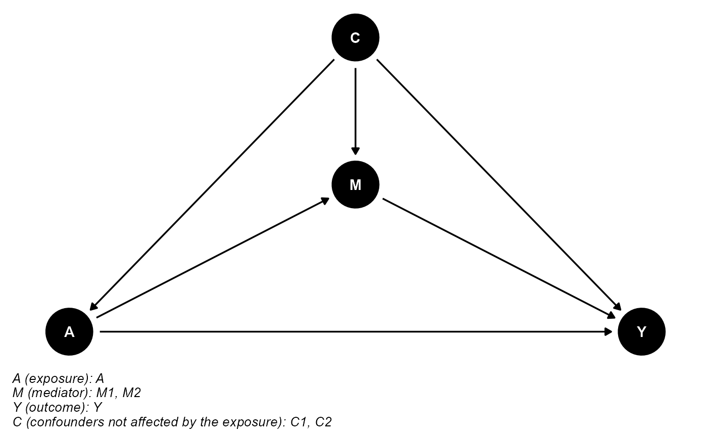
In this setting, we have a count mediator, so the marginal structural model is not available. We can use the rest five statistical modeling approaches. The results are shown below.
The Regression-based Approach
res_rb <- cmest(data = data, model = "rb", outcome = "Y", exposure = "A",
                mediator = c("M1", "M2"), basec = c("C1", "C2"), EMint = TRUE,
                mreg = list("poisson", "multinomial"), yreg = "logistic",
                astar = 0, a = 1, mval = list(0, 2),
                estimation = "imputation", inference = "bootstrap", nboot = 2)
summary(res_rb)## Causal Mediation Analysis
##
## # Outcome regression:
##
## Call:
## glm(formula = Y ~ A + M1 + M2 + A * M1 + A * M2 + C1 + C2, family = binomial(),
## data = getCall(x$reg.output$yreg)$data, weights = getCall(x$reg.output$yreg)$weights)
##
## Deviance Residuals:
## Min 1Q Median 3Q Max
## -2.2066 -0.5055 -0.0007 0.6383 3.3715
##
## Coefficients:
## Estimate Std. Error z value Pr(>|z|)
## (Intercept) 1.125104 0.478893 2.349 0.018804 *
## A 0.460265 0.400463 1.149 0.250419
## M1 -1.809307 0.180027 -10.050 < 2e-16 ***
## M21 -0.007101 0.364067 -0.020 0.984438
## M22 0.841167 0.405154 2.076 0.037879 *
## C1 0.504243 0.284671 1.771 0.076508 .
## C2 -0.643001 0.062025 -10.367 < 2e-16 ***
## A:M1 0.535812 0.183808 2.915 0.003556 **
## A:M21 0.129896 0.370967 0.350 0.726222
## A:M22 -1.447096 0.412172 -3.511 0.000447 ***
## ---
## Signif. codes: 0 '***' 0.001 '**' 0.01 '*' 0.05 '.' 0.1 ' ' 1
##
## (Dispersion parameter for binomial family taken to be 1)
##
## Null deviance: 13336.6 on 9999 degrees of freedom
## Residual deviance: 7347.9 on 9990 degrees of freedom
## AIC: 7367.9
##
## Number of Fisher Scoring iterations: 10
##
##
## # Mediator regressions:
##
## Call:
## glm(formula = M1 ~ A + C1 + C2, family = poisson(), data = getCall(x$reg.output$mreg[[1L]])$data,
## weights = getCall(x$reg.output$mreg[[1L]])$weights)
##
## Deviance Residuals:
## Min 1Q Median 3Q Max
## -3.4516 -1.0946 -0.2769 0.5079 3.4944
##
## Coefficients:
## Estimate Std. Error z value Pr(>|z|)
## (Intercept) 1.06240 0.05631 18.868 < 2e-16 ***
## A -2.00634 0.01331 -150.709 < 2e-16 ***
## C1 0.45102 0.05496 8.206 2.29e-16 ***
## C2 0.80084 0.01314 60.961 < 2e-16 ***
## ---
## Signif. codes: 0 '***' 0.001 '**' 0.01 '*' 0.05 '.' 0.1 ' ' 1
##
## (Dispersion parameter for poisson family taken to be 1)
##
## Null deviance: 43205 on 9999 degrees of freedom
## Residual deviance: 10846 on 9996 degrees of freedom
## AIC: 33081
##
## Number of Fisher Scoring iterations: 5
##
##
## Call:
## nnet::multinom(formula = M2 ~ A + C1 + C2, data = getCall(x$reg.output$mreg[[2]])$data,
## trace = FALSE, weights = getCall(x$reg.output$mreg[[2]])$weights)
##
## Coefficients:
## (Intercept) A C1 C2
## 1 1.946698 -1.785773 -0.3220412 0.7256062
## 2 0.654218 0.688984 -1.7259629 0.4295399
##
## Std. Errors:
## (Intercept) A C1 C2
## 1 0.2620667 0.06393051 0.2550181 0.05235024
## 2 0.3129261 0.10149606 0.2996053 0.06106820
##
## Residual Deviance: 17966.15
## AIC: 17982.15
##
## # Effect decomposition on the odds ratio scale via the regression-based approach
##
## Direct counterfactual imputation estimation with
## bootstrap standard errors, percentile confidence intervals and p-values
##
## Estimate Std.error 95% CIL 95% CIU P.val
## Rcde 0.377584 0.210028 0.124803 0.405 <2e-16 ***
## Rpnde 2.627088 0.263412 2.268273 2.622 <2e-16 ***
## Rtnde 1.460973 0.334983 1.054599 1.504 <2e-16 ***
## Rpnie 41.072338 8.052787 40.529554 51.346 <2e-16 ***
## Rtnie 22.841102 0.461080 23.252971 23.872 <2e-16 ***
## Rte 60.005575 5.079004 54.149180 60.972 <2e-16 ***
## ERcde -6.683723 1.717727 -8.708034 -6.400 <2e-16 ***
## ERintref 8.310810 1.454315 8.023107 9.977 <2e-16 ***
## ERintmed 17.306149 12.868379 1.509260 18.798 <2e-16 ***
## ERpnie 40.072338 8.052787 39.562749 50.382 <2e-16 ***
## ERcde(prop) -0.113273 0.042524 -0.164006 -0.107 <2e-16 ***
## ERintref(prop) 0.140848 0.040152 0.133921 0.188 <2e-16 ***
## ERintmed(prop) 0.293297 0.212212 0.027403 0.313 <2e-16 ***
## ERpnie(prop) 0.679128 0.214583 0.660446 0.949 <2e-16 ***
## pm 0.972425 0.002371 0.972955 0.976 <2e-16 ***
## int 0.434145 0.172059 0.215268 0.446 <2e-16 ***
## pe 1.113273 0.042524 1.106876 1.164 <2e-16 ***
## ---
## Signif. codes: 0 '***' 0.001 '**' 0.01 '*' 0.05 '.' 0.1 ' ' 1
##
## (Rcde: controlled direct effect odds ratio; Rpnde: pure natural direct effect odds ratio; Rtnde: total natural direct effect odds ratio; Rpnie: pure natural indirect effect odds ratio; Rtnie: total natural indirect effect odds ratio; Rte: total effect odds ratio; ERcde: excess relative risk due to controlled direct effect; ERintref: excess relative risk due to reference interaction; ERintmed: excess relative risk due to mediated interaction; ERpnie: excess relative risk due to pure natural indirect effect; ERcde(prop): proportion ERcde; ERintref(prop): proportion ERintref; ERintmed(prop): proportion ERintmed; ERpnie(prop): proportion ERpnie; pm: overall proportion mediated; int: overall proportion attributable to interaction; pe: overall proportion eliminated)
##
## Relevant variable values:
## $a
## [1] 1
##
## $astar
## [1] 0
##
## $yval
## [1] "1"
##
## $mval
## $mval[[1]]
## [1] 0
##
## $mval[[2]]
## [1] 2The Weighting-based Approach
res_wb <- cmest(data = data, model = "wb", outcome = "Y", exposure = "A",
                mediator = c("M1", "M2"), basec = c("C1", "C2"), EMint = TRUE,
                ereg = "logistic", yreg = "logistic",
                astar = 0, a = 1, mval = list(0, 2),
                estimation = "imputation", inference = "bootstrap", nboot = 2)
summary(res_wb)## Causal Mediation Analysis
##
## # Outcome regression:
##
## Call:
## glm(formula = Y ~ A + M1 + M2 + A * M1 + A * M2 + C1 + C2, family = binomial(),
## data = getCall(x$reg.output$yreg)$data, weights = getCall(x$reg.output$yreg)$weights)
##
## Deviance Residuals:
## Min 1Q Median 3Q Max
## -2.2066 -0.5055 -0.0007 0.6383 3.3715
##
## Coefficients:
## Estimate Std. Error z value Pr(>|z|)
## (Intercept) 1.125104 0.478893 2.349 0.018804 *
## A 0.460265 0.400463 1.149 0.250419
## M1 -1.809307 0.180027 -10.050 < 2e-16 ***
## M21 -0.007101 0.364067 -0.020 0.984438
## M22 0.841167 0.405154 2.076 0.037879 *
## C1 0.504243 0.284671 1.771 0.076508 .
## C2 -0.643001 0.062025 -10.367 < 2e-16 ***
## A:M1 0.535812 0.183808 2.915 0.003556 **
## A:M21 0.129896 0.370967 0.350 0.726222
## A:M22 -1.447096 0.412172 -3.511 0.000447 ***
## ---
## Signif. codes: 0 '***' 0.001 '**' 0.01 '*' 0.05 '.' 0.1 ' ' 1
##
## (Dispersion parameter for binomial family taken to be 1)
##
## Null deviance: 13336.6 on 9999 degrees of freedom
## Residual deviance: 7347.9 on 9990 degrees of freedom
## AIC: 7367.9
##
## Number of Fisher Scoring iterations: 10
##
##
## # Exposure regression for weighting:
##
## Call:
## glm(formula = A ~ C1 + C2, family = binomial(), data = getCall(x$reg.output$ereg)$data,
## weights = getCall(x$reg.output$ereg)$weights)
##
## Deviance Residuals:
## Min 1Q Median 3Q Max
## -1.6126 -1.4791 0.8573 0.8867 0.9750
##
## Coefficients:
## Estimate Std. Error z value Pr(>|z|)
## (Intercept) 0.08342 0.21440 0.389 0.69723
## C1 0.60899 0.21208 2.872 0.00409 **
## C2 0.10532 0.04375 2.407 0.01606 *
## ---
## Signif. codes: 0 '***' 0.001 '**' 0.01 '*' 0.05 '.' 0.1 ' ' 1
##
## (Dispersion parameter for binomial family taken to be 1)
##
## Null deviance: 12534 on 9999 degrees of freedom
## Residual deviance: 12520 on 9997 degrees of freedom
## AIC: 12526
##
## Number of Fisher Scoring iterations: 4
##
##
## # Effect decomposition on the odds ratio scale via the weighting-based approach
##
## Direct counterfactual imputation estimation with
## bootstrap standard errors, percentile confidence intervals and p-values
##
## Estimate Std.error 95% CIL 95% CIU P.val
## Rcde 0.3775843 0.0227470 0.3752670 0.406 <2e-16 ***
## Rpnde 2.2468828 0.1302465 2.1177910 2.293 <2e-16 ***
## Rtnde 1.4481237 0.0423478 1.3086198 1.366 <2e-16 ***
## Rpnie 37.2271375 2.3490397 35.1601269 38.316 <2e-16 ***
## Rtnie 23.9930181 0.8142279 21.7260533 22.820 <2e-16 ***
## Rte 53.9094991 4.6968302 46.0112396 52.321 <2e-16 ***
## ERcde -6.1503170 0.5444024 -5.7823835 -5.051 <2e-16 ***
## ERintref 7.3971997 0.6746489 6.1689534 7.075 <2e-16 ***
## ERintmed 15.4354789 2.2175440 9.7402420 12.720 <2e-16 ***
## ERpnie 36.2271375 2.3490397 34.1637376 37.320 <2e-16 ***
## ERcde(prop) -0.1162422 0.0003405 -0.1126449 -0.112 <2e-16 ***
## ERintref(prop) 0.1398085 0.0006058 0.1370179 0.138 <2e-16 ***
## ERintmed(prop) 0.2917336 0.0234156 0.2162252 0.248 <2e-16 ***
## ERpnie(prop) 0.6847001 0.0236809 0.7271290 0.759 <2e-16 ***
## pm 0.9764337 0.0002654 0.9748130 0.975 <2e-16 ***
## int 0.4315421 0.0240214 0.3532431 0.386 <2e-16 ***
## pe 1.1162422 0.0003405 1.1121875 1.113 <2e-16 ***
## ---
## Signif. codes: 0 '***' 0.001 '**' 0.01 '*' 0.05 '.' 0.1 ' ' 1
##
## (Rcde: controlled direct effect odds ratio; Rpnde: pure natural direct effect odds ratio; Rtnde: total natural direct effect odds ratio; Rpnie: pure natural indirect effect odds ratio; Rtnie: total natural indirect effect odds ratio; Rte: total effect odds ratio; ERcde: excess relative risk due to controlled direct effect; ERintref: excess relative risk due to reference interaction; ERintmed: excess relative risk due to mediated interaction; ERpnie: excess relative risk due to pure natural indirect effect; ERcde(prop): proportion ERcde; ERintref(prop): proportion ERintref; ERintmed(prop): proportion ERintmed; ERpnie(prop): proportion ERpnie; pm: overall proportion mediated; int: overall proportion attributable to interaction; pe: overall proportion eliminated)
##
## Relevant variable values:
## $a
## [1] 1
##
## $astar
## [1] 0
##
## $yval
## [1] "1"
##
## $mval
## $mval[[1]]
## [1] 0
##
## $mval[[2]]
## [1] 2The Inverse Odds-ratio Weighting Approach
res_iorw <- cmest(data = data, model = "iorw", outcome = "Y", exposure = "A",
                  mediator = c("M1", "M2"), basec = c("C1", "C2"), EMint = TRUE,
                  ereg = "logistic", yreg = "logistic",
                  astar = 0, a = 1, mval = list(0, 2),
                  estimation = "imputation", inference = "bootstrap", nboot = 2)
summary(res_iorw)## Causal Mediation Analysis
##
## # Outcome regression for the total effect:
##
## Call:
## glm(formula = Y ~ A + C1 + C2, family = binomial(), data = getCall(x$reg.output$yregTot)$data,
## weights = getCall(x$reg.output$yregTot)$weights)
##
## Deviance Residuals:
## Min 1Q Median 3Q Max
## -1.6731 -1.0673 -0.1524 0.7688 2.5278
##
## Coefficients:
## Estimate Std. Error z value Pr(>|z|)
## (Intercept) -2.9946 0.2726 -10.987 <2e-16 ***
## A 4.1997 0.1205 34.855 <2e-16 ***
## C1 -0.1306 0.2473 -0.528 0.597
## C2 -1.3288 0.0534 -24.885 <2e-16 ***
## ---
## Signif. codes: 0 '***' 0.001 '**' 0.01 '*' 0.05 '.' 0.1 ' ' 1
##
## (Dispersion parameter for binomial family taken to be 1)
##
## Null deviance: 13336.6 on 9999 degrees of freedom
## Residual deviance: 9397.2 on 9996 degrees of freedom
## AIC: 9405.2
##
## Number of Fisher Scoring iterations: 6
##
##
## # Outcome regression for the direct effect:
##
## Call:
## glm(formula = Y ~ A + C1 + C2, family = binomial(), data = getCall(x$reg.output$yregDir)$data,
## weights = getCall(x$reg.output$yregDir)$weights)
##
## Deviance Residuals:
## Min 1Q Median 3Q Max
## -4.7789 -0.0549 -0.0069 0.0818 8.4799
##
## Coefficients:
## Estimate Std. Error z value Pr(>|z|)
## (Intercept) -1.5600 0.7405 -2.107 0.0351 *
## A 1.7294 0.1460 11.848 <2e-16 ***
## C1 -1.2645 0.7413 -1.706 0.0880 .
## C2 -3.7661 0.4333 -8.691 <2e-16 ***
## ---
## Signif. codes: 0 '***' 0.001 '**' 0.01 '*' 0.05 '.' 0.1 ' ' 1
##
## (Dispersion parameter for binomial family taken to be 1)
##
## Null deviance: 1926.6 on 9999 degrees of freedom
## Residual deviance: 1423.0 on 9996 degrees of freedom
## AIC: 1214.1
##
## Number of Fisher Scoring iterations: 8
##
##
## # Exposure regression for weighting:
##
## Call:
## glm(formula = A ~ M1 + M2 + C1 + C2, family = binomial(), data = getCall(x$reg.output$ereg)$data,
## weights = getCall(x$reg.output$ereg)$weights)
##
## Deviance Residuals:
## Min 1Q Median 3Q Max
## -3.6520 -0.0024 0.0343 0.1447 3.1329
##
## Coefficients:
## Estimate Std. Error z value Pr(>|z|)
## (Intercept) 1.14163 0.58304 1.958 0.0502 .
## M1 -2.00321 0.05823 -34.402 < 2e-16 ***
## M21 0.08020 0.13700 0.585 0.5583
## M22 -0.01835 0.17781 -0.103 0.9178
## C1 3.43446 0.58316 5.889 3.88e-09 ***
## C2 4.84059 0.18684 25.907 < 2e-16 ***
## ---
## Signif. codes: 0 '***' 0.001 '**' 0.01 '*' 0.05 '.' 0.1 ' ' 1
##
## (Dispersion parameter for binomial family taken to be 1)
##
## Null deviance: 12534.4 on 9999 degrees of freedom
## Residual deviance: 2139.2 on 9994 degrees of freedom
## AIC: 2151.2
##
## Number of Fisher Scoring iterations: 8
##
##
## # Effect decomposition on the odds ratio scale via the inverse odds ratio weighting approach
##
## Direct counterfactual imputation estimation with
## bootstrap standard errors, percentile confidence intervals and p-values
##
## Estimate Std.error 95% CIL 95% CIU P.val
## Rte 52.434074 4.686177 54.249690 60.545 <2e-16 ***
## Rpnde 4.974916 0.521379 4.560246 5.261 <2e-16 ***
## Rtnie 10.539691 0.288168 11.509069 11.896 <2e-16 ***
## pm 0.922718 0.003494 0.928448 0.933 <2e-16 ***
## ---
## Signif. codes: 0 '***' 0.001 '**' 0.01 '*' 0.05 '.' 0.1 ' ' 1
##
## (Rte: total effect odds ratio; Rpnde: pure natural direct effect odds ratio; Rtnie: total natural indirect effect odds ratio; pm: proportion mediated)
##
## Relevant variable values:
## $a
## [1] 1
##
## $astar
## [1] 0
##
## $yval
## [1] "1"
{r message=F,warning=F,results='hide'} # res_ne <- cmest(data = data, model = "ne", outcome = "Y", exposure = "A", # mediator = c("M1", "M2"), basec = c("C1", "C2"), EMint = TRUE, # yreg = "logistic", # astar = 0, a = 1, mval = list(0, 2), # estimation = "imputation", inference = "bootstrap", nboot = 2) #
{r message=F,warning=F} # summary(res_ne) #
The g-formula Approach
res_gformula <- cmest(data = data, model = "gformula", outcome = "Y", exposure = "A",
                      mediator = c("M1", "M2"), basec = c("C1", "C2"), EMint = TRUE,
                      mreg = list("poisson", "multinomial"), yreg = "logistic",
                      astar = 0, a = 1, mval = list(0, 2),
                      estimation = "imputation", inference = "bootstrap", nboot = 2)
summary(res_gformula)## Causal Mediation Analysis
##
## # Outcome regression:
##
## Call:
## glm(formula = Y ~ A + M1 + M2 + A * M1 + A * M2 + C1 + C2, family = binomial(),
## data = getCall(x$reg.output$yreg)$data, weights = getCall(x$reg.output$yreg)$weights)
##
## Deviance Residuals:
## Min 1Q Median 3Q Max
## -2.2066 -0.5055 -0.0007 0.6383 3.3715
##
## Coefficients:
## Estimate Std. Error z value Pr(>|z|)
## (Intercept) 1.125104 0.478893 2.349 0.018804 *
## A 0.460265 0.400463 1.149 0.250419
## M1 -1.809307 0.180027 -10.050 < 2e-16 ***
## M21 -0.007101 0.364067 -0.020 0.984438
## M22 0.841167 0.405154 2.076 0.037879 *
## C1 0.504243 0.284671 1.771 0.076508 .
## C2 -0.643001 0.062025 -10.367 < 2e-16 ***
## A:M1 0.535812 0.183808 2.915 0.003556 **
## A:M21 0.129896 0.370967 0.350 0.726222
## A:M22 -1.447096 0.412172 -3.511 0.000447 ***
## ---
## Signif. codes: 0 '***' 0.001 '**' 0.01 '*' 0.05 '.' 0.1 ' ' 1
##
## (Dispersion parameter for binomial family taken to be 1)
##
## Null deviance: 13336.6 on 9999 degrees of freedom
## Residual deviance: 7347.9 on 9990 degrees of freedom
## AIC: 7367.9
##
## Number of Fisher Scoring iterations: 10
##
##
## # Mediator regressions:
##
## Call:
## glm(formula = M1 ~ A + C1 + C2, family = poisson(), data = getCall(x$reg.output$mreg[[1L]])$data,
## weights = getCall(x$reg.output$mreg[[1L]])$weights)
##
## Deviance Residuals:
## Min 1Q Median 3Q Max
## -3.4516 -1.0946 -0.2769 0.5079 3.4944
##
## Coefficients:
## Estimate Std. Error z value Pr(>|z|)
## (Intercept) 1.06240 0.05631 18.868 < 2e-16 ***
## A -2.00634 0.01331 -150.709 < 2e-16 ***
## C1 0.45102 0.05496 8.206 2.29e-16 ***
## C2 0.80084 0.01314 60.961 < 2e-16 ***
## ---
## Signif. codes: 0 '***' 0.001 '**' 0.01 '*' 0.05 '.' 0.1 ' ' 1
##
## (Dispersion parameter for poisson family taken to be 1)
##
## Null deviance: 43205 on 9999 degrees of freedom
## Residual deviance: 10846 on 9996 degrees of freedom
## AIC: 33081
##
## Number of Fisher Scoring iterations: 5
##
##
## Call:
## nnet::multinom(formula = M2 ~ A + C1 + C2, data = getCall(x$reg.output$mreg[[2]])$data,
## trace = FALSE, weights = getCall(x$reg.output$mreg[[2]])$weights)
##
## Coefficients:
## (Intercept) A C1 C2
## 1 1.946698 -1.785773 -0.3220412 0.7256062
## 2 0.654218 0.688984 -1.7259629 0.4295399
##
## Std. Errors:
## (Intercept) A C1 C2
## 1 0.2620667 0.06393051 0.2550181 0.05235024
## 2 0.3129261 0.10149606 0.2996053 0.06106820
##
## Residual Deviance: 17966.15
## AIC: 17982.15
##
## # Effect decomposition on the odds ratio scale via the g-formula approach
##
## Direct counterfactual imputation estimation with
## bootstrap standard errors, percentile confidence intervals and p-values
##
## Estimate Std.error 95% CIL 95% CIU P.val
## Rcde 0.3775843 0.0001090 0.5856582 0.586 <2e-16 ***
## Rpnde 2.6759571 0.0504529 2.6574057 2.725 <2e-16 ***
## Rtnde 1.4616207 0.0608864 1.5571605 1.639 <2e-16 ***
## Rpnie 44.5825480 4.3829136 35.3768867 41.265 <2e-16 ***
## Rtnie 24.3512032 2.1615388 21.2760736 24.180 <2e-16 ***
## Rte 65.1627748 4.6704478 57.9813237 64.256 <2e-16 ***
## ERcde -7.3006667 0.2990695 -4.4320239 -4.030 <2e-16 ***
## ERintref 8.9766238 0.2486166 5.7554354 6.089 <2e-16 ***
## ERintmed 18.9042697 0.3379871 20.8758549 21.330 <2e-16 ***
## ERpnie 43.5825480 4.3829136 34.3888139 40.277 <2e-16 ***
## ERcde(prop) -0.1137835 0.0004936 -0.0707202 -0.070 <2e-16 ***
## ERintref(prop) 0.1399039 0.0035268 0.0962663 0.101 <2e-16 ***
## ERintmed(prop) 0.2946299 0.0217063 0.3372324 0.366 <2e-16 ***
## ERpnie(prop) 0.6792497 0.0247395 0.6033208 0.637 <2e-16 ***
## pm 0.9738796 0.0030332 0.9697156 0.974 <2e-16 ***
## int 0.4345338 0.0252331 0.4334987 0.467 <2e-16 ***
## pe 1.1137835 0.0004936 1.0700571 1.071 <2e-16 ***
## ---
## Signif. codes: 0 '***' 0.001 '**' 0.01 '*' 0.05 '.' 0.1 ' ' 1
##
## (Rcde: controlled direct effect odds ratio; Rpnde: pure natural direct effect odds ratio; Rtnde: total natural direct effect odds ratio; Rpnie: pure natural indirect effect odds ratio; Rtnie: total natural indirect effect odds ratio; Rte: total effect odds ratio; ERcde: excess relative risk due to controlled direct effect; ERintref: excess relative risk due to reference interaction; ERintmed: excess relative risk due to mediated interaction; ERpnie: excess relative risk due to pure natural indirect effect; ERcde(prop): proportion ERcde; ERintref(prop): proportion ERintref; ERintmed(prop): proportion ERintmed; ERpnie(prop): proportion ERpnie; pm: overall proportion mediated; int: overall proportion attributable to interaction; pe: overall proportion eliminated)
##
## Relevant variable values:
## $a
## [1] 1
##
## $astar
## [1] 0
##
## $yval
## [1] "1"
##
## $mval
## $mval[[1]]
## [1] 0
##
## $mval[[2]]
## [1] 2