Statistical Modeling with Mediator-outcome Confounders Affected by the Exposure
2024-07-01
Source:vignettes/post_exposure_confounding.Rmd
post_exposure_confounding.RmdThis example demonstrates how to use cmest when there
are mediator-outcome confounders affected by the exposure. For this
purpose, we simulate some data containing a continuous baseline
confounder \(C_1\), a binary baseline
confounder \(C_2\), a binary exposure
\(A\), a continuous mediator-outcome
confounder affected by the exposure \(L\), a binary mediator \(M\) and a binary outcome \(Y\). The true regression models for \(A\), \(L\), \(M\)
and \(Y\) are: \[logit(E(A|C_1,C_2))=0.2+0.5C_1+0.1C_2\]
\[E(L|A,C_1,C_2)=1+A-C_1-0.5C_2\]
\[logit(E(M|A,L,C_1,C_2))=1+2A-L+1.5C_1+0.8C_2\]
\[logit(E(Y|A,L,M,C_1,C_2)))=-3-0.4A-1.2M+0.5AM-0.5L+0.3C_1-0.6C_2\]
set.seed(1)
expit <- function(x) exp(x)/(1+exp(x))
n <- 10000
C1 <- rnorm(n, mean = 1, sd = 0.1)
C2 <- rbinom(n, 1, 0.6)
A <- rbinom(n, 1, expit(0.2 + 0.5*C1 + 0.1*C2))
L <- rnorm(n, mean = 1 + A - C1 - 0.5*C2, sd = 0.5)
M <- rbinom(n, 1, expit(1 + 2*A - L + 1.5*C1 + 0.8*C2))
Y <- rbinom(n, 1, expit(-3 - 0.4*A - 1.2*M + 0.5*A*M - 0.5*L + 0.3*C1 - 0.6*C2))
data <- data.frame(A, M, Y, C1, C2, L)
The DAG for this scientific setting is:
## Registered S3 methods overwritten by 'lme4':
##   method                          from
##   cooks.distance.influence.merMod car
##   influence.merMod                car
##   dfbeta.influence.merMod         car
##   dfbetas.influence.merMod        car
cmdag(outcome = "Y", exposure = "A", mediator = "M",
      basec = c("C1", "C2"), postc = "L", node = TRUE, text_col = "white")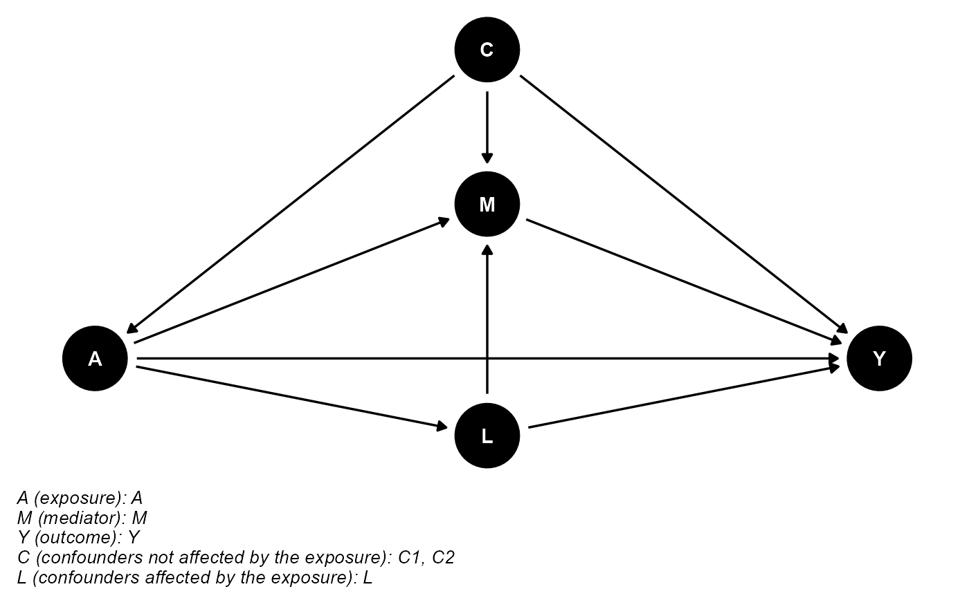
In this setting, we can use the marginal structural model and the \(g\)-formula approach. The results are shown below.
The Marginal Structural Model
res_msm <- cmest(data = data, model = "msm", outcome = "Y", exposure = "A",
                 mediator = "M", basec = c("C1", "C2"), postc = "L", EMint = TRUE,
                 ereg = "logistic", yreg = "logistic", mreg = list("logistic"),
                 wmnomreg = list("logistic"), wmdenomreg = list("logistic"),
                 astar = 0, a = 1, mval = list(1),
                 estimation = "imputation", inference = "bootstrap", nboot = 2)
summary(res_msm)## Causal Mediation Analysis
##
## # Outcome regression:
##
## Call:
## glm(formula = Y ~ A + M + A * M, family = binomial(), data = getCall(x$reg.output$yreg)$data,
## weights = getCall(x$reg.output$yreg)$weights)
##
## Deviance Residuals:
## Min 1Q Median 3Q Max
## -0.6465 -0.1964 -0.1428 -0.1399 3.3658
##
## Coefficients:
## Estimate Std. Error z value Pr(>|z|)
## (Intercept) -3.49700 0.47457 -7.369 1.72e-13 ***
## A 0.09466 0.67862 0.139 0.889
## M -0.40808 0.49218 -0.829 0.407
## A:M -0.79067 0.70198 -1.126 0.260
## ---
## Signif. codes: 0 '***' 0.001 '**' 0.01 '*' 0.05 '.' 0.1 ' ' 1
##
## (Dispersion parameter for binomial family taken to be 1)
##
## Null deviance: 1432.5 on 9999 degrees of freedom
## Residual deviance: 1412.9 on 9996 degrees of freedom
## AIC: 1432.5
##
## Number of Fisher Scoring iterations: 7
##
##
## # Mediator regressions:
##
## Call:
## glm(formula = M ~ A, family = binomial(), data = getCall(x$reg.output$mreg[[1L]])$data,
## weights = getCall(x$reg.output$mreg[[1L]])$weights)
##
## Deviance Residuals:
## Min 1Q Median 3Q Max
## -2.9114 0.1972 0.1999 0.3089 0.3437
##
## Coefficients:
## Estimate Std. Error z value Pr(>|z|)
## (Intercept) 2.96393 0.08185 36.211 < 2e-16 ***
## A 0.95266 0.11992 7.944 1.95e-15 ***
## ---
## Signif. codes: 0 '***' 0.001 '**' 0.01 '*' 0.05 '.' 0.1 ' ' 1
##
## (Dispersion parameter for binomial family taken to be 1)
##
## Null deviance: 2623.2 on 9999 degrees of freedom
## Residual deviance: 2560.6 on 9998 degrees of freedom
## AIC: 2580.5
##
## Number of Fisher Scoring iterations: 6
##
##
## # Mediator regressions for weighting (denominator):
##
## Call:
## glm(formula = M ~ A + C1 + C2 + L, family = binomial(), data = getCall(x$reg.output$wmdenomreg[[1L]])$data,
## weights = getCall(x$reg.output$wmdenomreg[[1L]])$weights)
##
## Deviance Residuals:
## Min 1Q Median 3Q Max
## -3.4241 0.1334 0.1885 0.2668 0.8260
##
## Coefficients:
## Estimate Std. Error z value Pr(>|z|)
## (Intercept) 0.9946 0.6067 1.639 0.1012
## A 1.8884 0.1726 10.944 < 2e-16 ***
## C1 1.4955 0.6090 2.456 0.0141 *
## C2 0.8166 0.1410 5.793 6.92e-09 ***
## L -0.9171 0.1215 -7.546 4.50e-14 ***
## ---
## Signif. codes: 0 '***' 0.001 '**' 0.01 '*' 0.05 '.' 0.1 ' ' 1
##
## (Dispersion parameter for binomial family taken to be 1)
##
## Null deviance: 2646.0 on 9999 degrees of freedom
## Residual deviance: 2397.3 on 9995 degrees of freedom
## AIC: 2407.3
##
## Number of Fisher Scoring iterations: 7
##
##
## # Mediator regressions for weighting (nominator):
##
## Call:
## glm(formula = M ~ A, family = binomial(), data = getCall(x$reg.output$wmnomreg[[1L]])$data,
## weights = getCall(x$reg.output$wmnomreg[[1L]])$weights)
##
## Deviance Residuals:
## Min 1Q Median 3Q Max
## -2.8106 0.1972 0.1972 0.3224 0.3224
##
## Coefficients:
## Estimate Std. Error z value Pr(>|z|)
## (Intercept) 2.93070 0.08064 36.345 <2e-16 ***
## A 0.99963 0.11952 8.364 <2e-16 ***
## ---
## Signif. codes: 0 '***' 0.001 '**' 0.01 '*' 0.05 '.' 0.1 ' ' 1
##
## (Dispersion parameter for binomial family taken to be 1)
##
## Null deviance: 2646.0 on 9999 degrees of freedom
## Residual deviance: 2576.3 on 9998 degrees of freedom
## AIC: 2580.3
##
## Number of Fisher Scoring iterations: 6
##
##
## # Exposure regression for weighting:
##
## Call:
## glm(formula = A ~ C1 + C2, family = binomial(), data = getCall(x$reg.output$ereg)$data,
## weights = getCall(x$reg.output$ereg)$weights)
##
## Deviance Residuals:
## Min 1Q Median 3Q Max
## -1.6126 -1.4791 0.8573 0.8867 0.9750
##
## Coefficients:
## Estimate Std. Error z value Pr(>|z|)
## (Intercept) 0.08342 0.21440 0.389 0.69723
## C1 0.60899 0.21208 2.872 0.00409 **
## C2 0.10532 0.04375 2.407 0.01606 *
## ---
## Signif. codes: 0 '***' 0.001 '**' 0.01 '*' 0.05 '.' 0.1 ' ' 1
##
## (Dispersion parameter for binomial family taken to be 1)
##
## Null deviance: 12534 on 9999 degrees of freedom
## Residual deviance: 12520 on 9997 degrees of freedom
## AIC: 12526
##
## Number of Fisher Scoring iterations: 4
##
##
## # Effect decomposition on the odds ratio scale via the marginal structural model
##
## Direct counterfactual imputation estimation with
## bootstrap standard errors, percentile confidence intervals and p-values
##
## Estimate Std.error 95% CIL 95% CIU P.val
## Rcde 0.498566 0.170135 0.389190 0.618 <2e-16 ***
## rRpnde 0.538980 0.183557 0.399533 0.646 <2e-16 ***
## rRtnde 0.516082 0.175401 0.393873 0.629 <2e-16 ***
## rRpnie 0.986900 0.008207 1.002534 1.014 <2e-16 ***
## rRtnie 0.944972 0.016691 0.976778 0.999 <2e-16 ***
## Rte 0.509321 0.172602 0.399214 0.631 <2e-16 ***
## ERcde -0.485305 0.179358 -0.619447 -0.378 <2e-16 ***
## rERintref 0.024285 0.004199 0.020452 0.026 <2e-16 ***
## rERintmed -0.016558 0.002748 -0.017719 -0.014 <2e-16 ***
## rERpnie -0.013100 0.008207 0.002535 0.014 <2e-16 ***
## ERcde(prop) 0.989048 0.002742 1.029616 1.033 <2e-16 ***
## rERintref(prop) -0.049493 0.027626 -0.071621 -0.035 <2e-16 ***
## rERintmed(prop) 0.033746 0.018586 0.023662 0.049 <2e-16 ***
## rERpnie(prop) 0.026698 0.011783 -0.022457 -0.007 <2e-16 ***
## rpm 0.060445 0.030369 0.001204 0.042 <2e-16 ***
## rint -0.015747 0.009040 -0.022989 -0.011 <2e-16 ***
## rpe 0.010952 0.002742 -0.033300 -0.030 <2e-16 ***
## ---
## Signif. codes: 0 '***' 0.001 '**' 0.01 '*' 0.05 '.' 0.1 ' ' 1
##
## (Rcde: controlled direct effect odds ratio; rRpnde: randomized analogue of pure natural direct effect odds ratio; rRtnde: randomized analogue of total natural direct effect odds ratio; rRpnie: randomized analogue of pure natural indirect effect odds ratio; rRtnie: randomized analogue of total natural indirect effect odds ratio; Rte: total effect odds ratio; ERcde: excess relative risk due to controlled direct effect; rERintref: randomized analogue of excess relative risk due to reference interaction; rERintmed: randomized analogue of excess relative risk due to mediated interaction; rERpnie: randomized analogue of excess relative risk due to pure natural indirect effect; ERcde(prop): proportion ERcde; rERintref(prop): proportion rERintref; rERintmed(prop): proportion rERintmed; rERpnie(prop): proportion rERpnie; rpm: randomized analogue of overall proportion mediated; rint: randomized analogue of overall proportion attributable to interaction; rpe: randomized analogue of overall proportion eliminated)
##
## Relevant variable values:
## $a
## [1] 1
##
## $astar
## [1] 0
##
## $yval
## [1] "1"
##
## $mval
## $mval[[1]]
## [1] 1The g-formula Approach
res_gformula <- cmest(data = data, model = "gformula", outcome = "Y", exposure = "A",
                      mediator = "M", basec = c("C1", "C2"), postc = "L", EMint = TRUE,
                      mreg = list("logistic"), yreg = "logistic", postcreg = list("linear"),
                      astar = 0, a = 1, mval = list(1),
                      estimation = "imputation", inference = "bootstrap", nboot = 2)
summary(res_gformula)## Causal Mediation Analysis
##
## # Outcome regression:
##
## Call:
## glm(formula = Y ~ A + M + A * M + C1 + C2 + L, family = binomial(),
## data = getCall(x$reg.output$yreg)$data, weights = getCall(x$reg.output$yreg)$weights)
##
## Deviance Residuals:
## Min 1Q Median 3Q Max
## -0.3617 -0.1788 -0.1545 -0.1289 3.1833
##
## Coefficients:
## Estimate Std. Error z value Pr(>|z|)
## (Intercept) -2.7488 0.9365 -2.935 0.00333 **
## A -0.1267 0.6617 -0.192 0.84812
## M -0.7274 0.4136 -1.759 0.07863 .
## C1 -0.1906 0.8705 -0.219 0.82664
## C2 -0.5566 0.1933 -2.880 0.00397 **
## L -0.2242 0.1709 -1.312 0.18964
## A:M -0.3425 0.6635 -0.516 0.60572
## ---
## Signif. codes: 0 '***' 0.001 '**' 0.01 '*' 0.05 '.' 0.1 ' ' 1
##
## (Dispersion parameter for binomial family taken to be 1)
##
## Null deviance: 1447.7 on 9999 degrees of freedom
## Residual deviance: 1415.5 on 9993 degrees of freedom
## AIC: 1429.5
##
## Number of Fisher Scoring iterations: 7
##
##
## # Mediator regressions:
##
## Call:
## glm(formula = M ~ A + C1 + C2 + L, family = binomial(), data = getCall(x$reg.output$mreg[[1L]])$data,
## weights = getCall(x$reg.output$mreg[[1L]])$weights)
##
## Deviance Residuals:
## Min 1Q Median 3Q Max
## -3.4241 0.1334 0.1885 0.2668 0.8260
##
## Coefficients:
## Estimate Std. Error z value Pr(>|z|)
## (Intercept) 0.9946 0.6067 1.639 0.1012
## A 1.8884 0.1726 10.944 < 2e-16 ***
## C1 1.4955 0.6090 2.456 0.0141 *
## C2 0.8166 0.1410 5.793 6.92e-09 ***
## L -0.9171 0.1215 -7.546 4.50e-14 ***
## ---
## Signif. codes: 0 '***' 0.001 '**' 0.01 '*' 0.05 '.' 0.1 ' ' 1
##
## (Dispersion parameter for binomial family taken to be 1)
##
## Null deviance: 2646.0 on 9999 degrees of freedom
## Residual deviance: 2397.3 on 9995 degrees of freedom
## AIC: 2407.3
##
## Number of Fisher Scoring iterations: 7
##
##
## # Regressions for mediator-outcome confounders affected by the exposure:
##
## Call:
## glm(formula = L ~ A + C1 + C2, family = gaussian(), data = getCall(x$reg.output$postcreg[[1L]])$data,
## weights = getCall(x$reg.output$postcreg[[1L]])$weights)
##
## Deviance Residuals:
## Min 1Q Median 3Q Max
## -1.82456 -0.34194 0.00712 0.33751 1.82462
##
## Coefficients:
## Estimate Std. Error t value Pr(>|t|)
## (Intercept) 1.00268 0.05077 19.75 <2e-16 ***
## A 1.00202 0.01081 92.68 <2e-16 ***
## C1 -1.00369 0.04980 -20.15 <2e-16 ***
## C2 -0.49437 0.01032 -47.92 <2e-16 ***
## ---
## Signif. codes: 0 '***' 0.001 '**' 0.01 '*' 0.05 '.' 0.1 ' ' 1
##
## (Dispersion parameter for gaussian family taken to be 0.2539334)
##
## Null deviance: 5324.2 on 9999 degrees of freedom
## Residual deviance: 2538.3 on 9996 degrees of freedom
## AIC: 14678
##
## Number of Fisher Scoring iterations: 2
##
##
## # Effect decomposition on the odds ratio scale via the g-formula approach
##
## Direct counterfactual imputation estimation with
## bootstrap standard errors, percentile confidence intervals and p-values
##
## Estimate Std.error 95% CIL 95% CIU P.val
## Rcde 0.499968 0.003306 0.627867 0.632 <2e-16 ***
## rRpnde 0.518971 0.062605 0.540497 0.625 <2e-16 ***
## rRtnde 0.508831 0.026424 0.593114 0.629 <2e-16 ***
## rRpnie 0.973863 0.030486 0.940677 0.982 <2e-16 ***
## rRtnie 0.954837 0.032978 0.987946 1.032 1
## Rte 0.495532 0.044022 0.557928 0.617 <2e-16 ***
## ERcde -0.471832 0.012399 -0.350420 -0.334 <2e-16 ***
## rERintref -0.009197 0.075004 -0.125581 -0.025 <2e-16 ***
## rERintmed 0.002698 0.049068 0.010726 0.077 <2e-16 ***
## rERpnie -0.026137 0.030486 -0.059300 -0.018 <2e-16 ***
## ERcde(prop) 0.935307 0.119282 0.755709 0.916 <2e-16 ***
## rERintref(prop) 0.018231 0.163331 0.063896 0.283 <2e-16 ***
## rERintmed(prop) -0.005349 0.108286 -0.172893 -0.027 <2e-16 ***
## rERpnie(prop) 0.051810 0.064238 0.047549 0.134 <2e-16 ***
## rpm 0.046462 0.044049 -0.039041 0.020 1
## rint 0.012883 0.055045 0.036486 0.110 <2e-16 ***
## rpe 0.064693 0.119282 0.084035 0.244 <2e-16 ***
## ---
## Signif. codes: 0 '***' 0.001 '**' 0.01 '*' 0.05 '.' 0.1 ' ' 1
##
## (Rcde: controlled direct effect odds ratio; rRpnde: randomized analogue of pure natural direct effect odds ratio; rRtnde: randomized analogue of total natural direct effect odds ratio; rRpnie: randomized analogue of pure natural indirect effect odds ratio; rRtnie: randomized analogue of total natural indirect effect odds ratio; Rte: total effect odds ratio; ERcde: excess relative risk due to controlled direct effect; rERintref: randomized analogue of excess relative risk due to reference interaction; rERintmed: randomized analogue of excess relative risk due to mediated interaction; rERpnie: randomized analogue of excess relative risk due to pure natural indirect effect; ERcde(prop): proportion ERcde; rERintref(prop): proportion rERintref; rERintmed(prop): proportion rERintmed; rERpnie(prop): proportion rERpnie; rpm: randomized analogue of overall proportion mediated; rint: randomized analogue of overall proportion attributable to interaction; rpe: randomized analogue of overall proportion eliminated)
##
## Relevant variable values:
## $a
## [1] 1
##
## $astar
## [1] 0
##
## $yval
## [1] "1"
##
## $mval
## $mval[[1]]
## [1] 1