Statistical Modeling for a Case Control Study
2024-07-01
Source:vignettes/case_control.Rmd
case_control.RmdThis example demonstrates how to use cmest for a case
control study. For this purpose, we simulate some data containing a
continuous baseline confounder \(C_1\),
a binary baseline confounder \(C_2\), a
binary exposure \(A\), a binary
mediator \(M\) and a binary outcome
\(Y\). We sample 2000 cases out of all
cases and sample 2000 controls out of all controls. The true regression
models for \(A\), \(M\) and \(Y\) are: \[logit(E(A|C_1,C_2))=0.2+0.5C_1+0.1C_2\]
\[logit(E(M|A,C_1,C_2))=1+2A+1.5C_1+0.8C_2\]
\[logit(E(Y|A,M,C_1,C_2)))=-5+0.8A-1.8M+0.5AM+0.3C_1-0.6C_2\]
set.seed(1)
# data simulation
expit <- function(x) exp(x)/(1+exp(x))
n <- 1000000
C1 <- rnorm(n, mean = 1, sd = 0.1)
C2 <- rbinom(n, 1, 0.6)
A <- rbinom(n, 1, expit(0.2 + 0.5*C1 + 0.1*C2))
M <- rbinom(n, 1, expit(1 + 2*A + 1.5*C1 + 0.8*C2))
Y <- rbinom(n, 1, expit(-5 + 0.8*A - 1.8*M + 0.5*A*M + 0.3*C1 - 0.6*C2))
yprevalence <- sum(Y)/n
data <- data.frame(A, M, Y, C1, C2)
case_indice <- sample(which(data$Y == 1), 2000, replace = FALSE)
control_indice <- sample(which(data$Y == 0), 2000, replace = FALSE)
data <- data[c(case_indice, control_indice), ]
The DAG for this scientific setting is:
## Registered S3 methods overwritten by 'lme4':
##   method                          from
##   cooks.distance.influence.merMod car
##   influence.merMod                car
##   dfbeta.influence.merMod         car
##   dfbetas.influence.merMod        car
cmdag(outcome = "Y", exposure = "A", mediator = "M",
      basec = c("C1", "C2"), postc = NULL, node = TRUE, text_col = "white")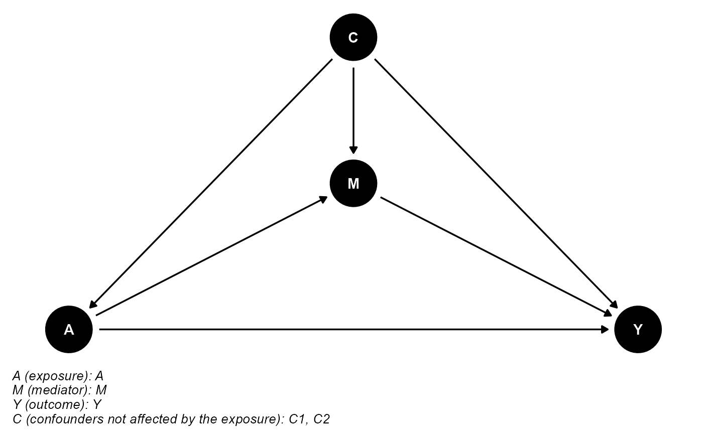
For a case control study, we set the casecontrol
argument to be TRUE. It requires that either the prevalence
of the case be known or the case be rare. We use the regression-based
approach for illustration.
If the prevalence of the case is known, we specify it by the
yprevalence argument. The results are:
res_yprevelence <- cmest(data = data, model = "rb", casecontrol = TRUE, yprevalence = yprevalence,
                         outcome = "Y", exposure = "A",
                         mediator = "M", basec = c("C1", "C2"), EMint = TRUE,
                         mreg = list("logistic"), yreg = "logistic",
                         astar = 0, a = 1, mval = list(1),
                         estimation = "paramfunc", inference = "delta")
summary(res_yprevelence)## Causal Mediation Analysis
##
## # Outcome regression:
##
## Call:
## svyglm(formula = Y ~ A + M + A * M + C1 + C2, design = getCall(x$reg.output$yreg)$design,
## family = getCall(x$reg.output$yreg)$family)
##
## Survey design:
## survey::svydesign(~1, data = getCall(x$reg.output.summary$yreg$survey.design)$data,
## weights = getCall(x$reg.output.summary$yreg$survey.design)$weights)
##
## Coefficients:
## Estimate Std. Error t value Pr(>|t|)
## (Intercept) -4.97446 0.39866 -12.478 < 2e-16 ***
## A 1.08507 0.39955 2.716 0.00664 **
## M -1.66061 0.22032 -7.537 5.9e-14 ***
## C1 0.14732 0.34430 0.428 0.66875
## C2 -0.61153 0.06887 -8.879 < 2e-16 ***
## A:M 0.19323 0.40922 0.472 0.63682
## ---
## Signif. codes: 0 '***' 0.001 '**' 0.01 '*' 0.05 '.' 0.1 ' ' 1
##
## (Dispersion parameter for binomial family taken to be 0.9919739)
##
## Number of Fisher Scoring iterations: 9
##
##
## # Mediator regressions:
##
## Call:
## svyglm(formula = M ~ A + C1 + C2, design = getCall(x$reg.output$mreg[[1L]])$design,
## family = getCall(x$reg.output$mreg[[1L]])$family)
##
## Survey design:
## survey::svydesign(~1, data = getCall(x$reg.output.summary$mreg[[1L]]$survey.design)$data,
## weights = getCall(x$reg.output.summary$mreg[[1L]]$survey.design)$weights)
##
## Coefficients:
## Estimate Std. Error t value Pr(>|t|)
## (Intercept) 0.7836 1.5384 0.509 0.6105
## A 1.9558 0.3439 5.687 1.38e-08 ***
## C1 1.6832 1.5600 1.079 0.2807
## C2 0.7054 0.2965 2.379 0.0174 *
## ---
## Signif. codes: 0 '***' 0.001 '**' 0.01 '*' 0.05 '.' 0.1 ' ' 1
##
## (Dispersion parameter for binomial family taken to be 1.045659)
##
## Number of Fisher Scoring iterations: 7
##
##
## # Effect decomposition on the odds ratio scale for a case control study via the regression-based approach
##
## Closed-form parameter function estimation with
## delta method standard errors, confidence intervals and p-values
##
## Estimate Std.error 95% CIL 95% CIU P.val
## Rcde 3.59054 0.31733 3.01948 4.270 < 2e-16 ***
## Rpnde 3.44231 0.37396 2.78213 4.259 < 2e-16 ***
## Rtnde 3.56427 0.30685 3.01087 4.219 < 2e-16 ***
## Rpnie 0.83794 0.04473 0.75471 0.930 0.000925 ***
## Rtnie 0.86763 0.05490 0.76644 0.982 0.024823 *
## Rte 2.98666 0.27610 2.49171 3.580 < 2e-16 ***
## ERcde 2.09752 0.25249 1.60265 2.592 < 2e-16 ***
## ERintref 0.34479 0.25148 -0.14810 0.838 0.170361
## ERintmed -0.29359 0.21623 -0.71740 0.130 0.174540
## ERpnie -0.16206 0.04473 -0.24972 -0.074 0.000291 ***
## ERcde(prop) 1.05580 0.03792 0.98148 1.130 < 2e-16 ***
## ERintref(prop) 0.17355 0.12318 -0.06788 0.415 0.158862
## ERintmed(prop) -0.14778 0.10636 -0.35624 0.061 0.164683
## ERpnie(prop) -0.08157 0.02901 -0.13843 -0.025 0.004921 **
## pm -0.22935 0.11082 -0.44656 -0.012 0.038494 *
## int 0.02577 0.01922 -0.01190 0.063 0.179931
## pe -0.05580 0.03792 -0.13013 0.019 0.141133
## ---
## Signif. codes: 0 '***' 0.001 '**' 0.01 '*' 0.05 '.' 0.1 ' ' 1
##
## (Rcde: controlled direct effect odds ratio; Rpnde: pure natural direct effect odds ratio; Rtnde: total natural direct effect odds ratio; Rpnie: pure natural indirect effect odds ratio; Rtnie: total natural indirect effect odds ratio; Rte: total effect odds ratio; ERcde: excess relative risk due to controlled direct effect; ERintref: excess relative risk due to reference interaction; ERintmed: excess relative risk due to mediated interaction; ERpnie: excess relative risk due to pure natural indirect effect; ERcde(prop): proportion ERcde; ERintref(prop): proportion ERintref; ERintmed(prop): proportion ERintmed; ERpnie(prop): proportion ERpnie; pm: overall proportion mediated; int: overall proportion attributable to interaction; pe: overall proportion eliminated)
##
## Relevant variable values:
## $a
## [1] 1
##
## $astar
## [1] 0
##
## $yval
## [1] "1"
##
## $mval
## $mval[[1]]
## [1] 1
##
##
## $basecval
## $basecval[[1]]
## [1] 1.002184
##
## $basecval[[2]]
## [1] 0.5255If the prevalence of the case is unknown but we know the case is
rare, we set the yrare argument to be TRUE.
The results are:
res_yrare <- cmest(data = data, model = "rb", casecontrol = TRUE, yrare = TRUE,
                   outcome = "Y", exposure = "A",
                   mediator = "M", basec = c("C1", "C2"), EMint = TRUE,
                   mreg = list("logistic"), yreg = "logistic",
                   astar = 0, a = 1, mval = list(1),
                   estimation = "paramfunc", inference = "delta")
summary(res_yrare)## Causal Mediation Analysis
##
## # Outcome regression:
##
## Call:
## glm(formula = Y ~ A + M + A * M + C1 + C2, family = binomial(),
## data = getCall(x$reg.output$yreg)$data, weights = getCall(x$reg.output$yreg)$weights)
##
## Deviance Residuals:
## Min 1Q Median 3Q Max
## -2.02664 -1.14853 -0.07283 1.04234 1.79068
##
## Coefficients:
## Estimate Std. Error z value Pr(>|z|)
## (Intercept) 0.87856 0.38849 2.261 0.0237 *
## A 0.96088 0.38782 2.478 0.0132 *
## M -1.69239 0.21731 -7.788 6.82e-15 ***
## C1 0.07022 0.33423 0.210 0.8336
## C2 -0.62047 0.06664 -9.310 < 2e-16 ***
## A:M 0.33475 0.39764 0.842 0.3999
## ---
## Signif. codes: 0 '***' 0.001 '**' 0.01 '*' 0.05 '.' 0.1 ' ' 1
##
## (Dispersion parameter for binomial family taken to be 1)
##
## Null deviance: 5545.2 on 3999 degrees of freedom
## Residual deviance: 5163.4 on 3994 degrees of freedom
## AIC: 5175.4
##
## Number of Fisher Scoring iterations: 4
##
##
## # Mediator regressions:
##
## Call:
## glm(formula = M ~ A + C1 + C2, family = binomial(), data = getCall(x$reg.output$mreg[[1L]])$data,
## weights = getCall(x$reg.output$mreg[[1L]])$weights)
##
## Deviance Residuals:
## Min 1Q Median 3Q Max
## -3.2695 0.1089 0.1460 0.2770 0.5010
##
## Coefficients:
## Estimate Std. Error z value Pr(>|z|)
## (Intercept) 0.7862 1.4552 0.540 0.5890
## A 1.9627 0.3474 5.650 1.6e-08 ***
## C1 1.6876 1.4587 1.157 0.2473
## C2 0.7016 0.2982 2.353 0.0186 *
## ---
## Signif. codes: 0 '***' 0.001 '**' 0.01 '*' 0.05 '.' 0.1 ' ' 1
##
## (Dispersion parameter for binomial family taken to be 1)
##
## Null deviance: 452.89 on 1999 degrees of freedom
## Residual deviance: 406.21 on 1996 degrees of freedom
## AIC: 414.21
##
## Number of Fisher Scoring iterations: 7
##
##
## # Effect decomposition on the odds ratio scale for a case control study via the regression-based approach
##
## Closed-form parameter function estimation with
## delta method standard errors, confidence intervals and p-values
##
## Estimate Std.error 95% CIL 95% CIU P.val
## Rcde 3.65329 0.32168 3.07422 4.341 < 2e-16 ***
## Rpnde 3.40407 0.35328 2.77754 4.172 < 2e-16 ***
## Rtnde 3.60919 0.30906 3.05155 4.269 < 2e-16 ***
## Rpnie 0.83319 0.04532 0.74893 0.927 0.000794 ***
## Rtnie 0.88340 0.04962 0.79131 0.986 0.027294 *
## Rte 3.00715 0.27763 2.50939 3.604 < 2e-16 ***
## ERcde 2.13416 0.25499 1.63438 2.634 < 2e-16 ***
## ERintref 0.26991 0.21978 -0.16085 0.701 0.219412
## ERintmed -0.23012 0.18887 -0.60029 0.140 0.223076
## ERpnie -0.16681 0.04532 -0.25564 -0.078 0.000233 ***
## ERcde(prop) 1.06328 0.03649 0.99175 1.135 < 2e-16 ***
## ERintref(prop) 0.13447 0.10691 -0.07507 0.344 0.208453
## ERintmed(prop) -0.11465 0.09217 -0.29530 0.066 0.213549
## ERpnie(prop) -0.08311 0.02927 -0.14047 -0.026 0.004517 **
## pm -0.19776 0.09648 -0.38686 -0.009 0.040401 *
## int 0.01983 0.01642 -0.01235 0.052 0.227195
## pe -0.06328 0.03649 -0.13481 0.008 0.082916 .
## ---
## Signif. codes: 0 '***' 0.001 '**' 0.01 '*' 0.05 '.' 0.1 ' ' 1
##
## (Rcde: controlled direct effect odds ratio; Rpnde: pure natural direct effect odds ratio; Rtnde: total natural direct effect odds ratio; Rpnie: pure natural indirect effect odds ratio; Rtnie: total natural indirect effect odds ratio; Rte: total effect odds ratio; ERcde: excess relative risk due to controlled direct effect; ERintref: excess relative risk due to reference interaction; ERintmed: excess relative risk due to mediated interaction; ERpnie: excess relative risk due to pure natural indirect effect; ERcde(prop): proportion ERcde; ERintref(prop): proportion ERintref; ERintmed(prop): proportion ERintmed; ERpnie(prop): proportion ERpnie; pm: overall proportion mediated; int: overall proportion attributable to interaction; pe: overall proportion eliminated)
##
## Relevant variable values:
## $a
## [1] 1
##
## $astar
## [1] 0
##
## $yval
## [1] "1"
##
## $mval
## $mval[[1]]
## [1] 1
##
##
## $basecval
## $basecval[[1]]
## [1] 1.002184
##
## $basecval[[2]]
## [1] 0.5255