Multistate approach for stochastic interventions on a time-to event mediator in the presence of competing risks

The DAG for this scientific setting is as follows:

cmdag(outcome = "S", exposure = "A", mediator = "M",
      basec = c("C1", "C2"), postc = NULL, node = TRUE, text_col = "white")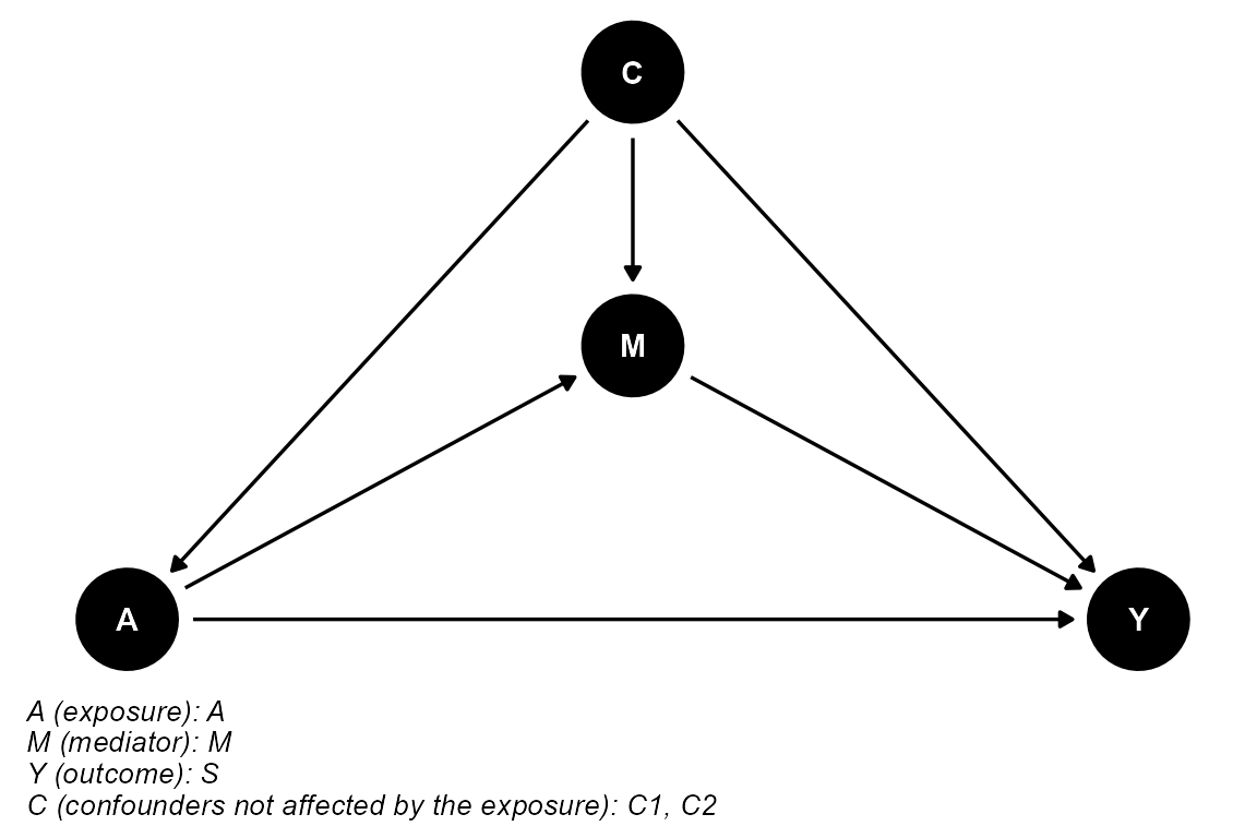

An example is given to demonstrate how to use cmest_multistate when there is a time-to-event mediator and a time-to-event outcome, and the estimation of RD and SD is of interest. For this purpose, we simulate a dataset with a binary exposure A, a time-to-event mediator M, a timeto-event outcome S, and two baseline covariates: one continuous (C1), and one binary (C2).

Data simulation

We simulate data following the structure shown in the above DAG. Specifically, we separately generate the following transitions under a Cox proportional hazards model with the constant baseline hazard, i.e., assuming exponential time to event:

Transition 1 (\(A \rightarrow M\)): \(\lambda_{01}(t|A,C1,C2) = \lambda_{01}^0(t)e^{a_1A+a_2C1+a_3C2} = 1.5 \cdot e^{=1.9A+0.2C1+0.5C2}\)
Transition 2 (\(A \rightarrow S\)): \(\lambda_{02}(t|A,C1,C2) = \lambda_{02}^0(t)e^{b_1A+b_3C1+b_4C2} = 1 \cdot e^{A-0.5C1-0.3C2}\)
Transition 3 (\(M \rightarrow S\)): \(\lambda_{12}(t|A,C1,C2) = \lambda_{12}^0(t)e^{c_1A+c_2M+c_3C1+c_4C2} = 0.8 \cdot e^{0.55A-0.15M -0.1C1-0.2C2}\)

The code for generating the aforementioned data is as follows:

# set up coefficients 
# transition 1 (A to M)
a1 = -1.9 
a2 = 0.2 
a3 = 0.5 

# transition 2 (A to S)
b1 = 1 
b3 = -0.5
b4 = 0.3

# transition 3 (M to S)
c1 = 0.55
c2 = -0.15 
c3 = -0.1 
c4 = -0.2 

set.seed(8) 

# build a function to generate time-to-event data
gen_srv <- function(n, lambda, beta, X){
  X = as.matrix(X)
  beta = as.matrix(beta, ncol=1)
  time = -log(runif(n)) / (lambda * exp(X %*% beta)) 
  return(time)
}

n <- 2000 
A = sample(c(0,1),replace=TRUE, size=n, c(0.5,0.5)) #binary exposure
C1 = sample(c(0,1),replace=TRUE, size=n,c(0.6, 0.4)) #binary baseline covariate
C2 = rnorm(n, mean = 1, sd = 1) #continuous baseline covariate
id=c(1:n)
full = data.frame(id,A,C1,C2)
M = gen_srv(n=n, lambda = 1.5, beta = c(a1,a2,a3), X=data.frame(A,C1,C2)) #time to event mediator
S = gen_srv(n=n, lambda = 1, beta = c(b1,b3,b4), X=data.frame(A,C1,C2)) #time to event outcome
data = data.frame(id = c(1:n), M = M, S = S)
# indicator for event
data$ind_M = ifelse(data$M <= data$S, 1, 0)
data$ind_S = 1
data <- merge(data,full , by = "id")
# modify S distribution
trans_matrix = transMat(x = list(c(2, 3), c(3), c()), names = c("A", "M", "S"))
covs = c("A","M", "C1","C2")
pre_data = msprep(time = c(NA, "M", "S"), status = c(NA, "ind_M", "ind_S"),
                         data = data, trans = trans_matrix, keep = covs)
pre_data = expand.covs(pre_data, covs, append = TRUE, longnames = FALSE)
# resample for T < S
data_23 = pre_data[which(pre_data$trans == 3),]
data_23_tem = data.frame(id = rep(NA,dim(data_23)[1]),
                         new_y = rep(NA,dim(data_23)[1]))
paste("# to resample is ", nrow(data_23))

## [1] "# to resample is  823"

for(i in 1:dim(data_23)[1]){
  data_23_tem$id[i] = data_23$id[i]
  repeat {
    time_test = gen_srv(n = 1, 
                        lambda = 0.8,
                        beta = c(as.numeric(c1),
                                 c2,
                                 as.numeric(c3),
                                 as.numeric(c4)), 
                        X = data_23[i, c("A.3", "M.3", "C1.3","C2.3")])
    # exit if the condition is met
    if (time_test > data_23[i,"M.3"]) break
  }
  data_23_tem$new_y[i] = time_test
}
data_temp = merge(data, data_23_tem, by = "id", all = T)
# modify M and S
data_temp$S[which(data_temp$ind_M == 1)] = data_temp$new_y[which(data_temp$ind_M == 1)]
data_temp$M[which(data_temp$ind_M == 0)] = data_temp$S[which(data_temp$ind_M == 0)]
data_final = data_temp
data_final$A = as.factor(data_final$A) 

sc_data = data_final %>% dplyr::select(id,A,M,S,ind_M,ind_S,C1,C2)

# generate time to censoring and update event indicator
time_to_censor = runif(n, 0, 2*max(sc_data$S))
sc_data$ind_S = ifelse(sc_data$S > time_to_censor, 0, 1)
sc_data$A = factor(sc_data$A)
sc_data$C1 = factor(sc_data$C1)

We fit the multistate Cox proportional hazards model to the simulated data. We can see that the regression coefficient estimates are close to the set-up values, which is expected:

## prepare the simulated data into counting process format
mstate_sc_data = msprep(time = c(NA, "M", "S"), status = c(NA, "ind_M", "ind_S"),
                         data = sc_data, trans = trans_matrix, keep = covs)
mstate_sc_data = expand.covs(mstate_sc_data, covs, append = TRUE, longnames = FALSE)

## fit mstate model to the simulated data
sc_joint_mod = coxph(Surv(Tstart, Tstop, status) ~ A.1 + A.2 + A.3 +
                         M.3 + C1.1 + C1.2 + C1.3 + C2.1 + C2.2 + C2.3 + strata(trans),
                      data = mstate_sc_data)
summary(sc_joint_mod)

## Call:
## coxph(formula = Surv(Tstart, Tstop, status) ~ A.1 + A.2 + A.3 + 
##     M.3 + C1.1 + C1.2 + C1.3 + C2.1 + C2.2 + C2.3 + strata(trans), 
##     data = mstate_sc_data)
## 
##   n= 4823, number of events= 2746 
## 
##          coef exp(coef) se(coef)       z Pr(>|z|)    
## A.1  -1.82713   0.16088  0.09545 -19.143  < 2e-16 ***
## A.2   0.95419   2.59658  0.06776  14.081  < 2e-16 ***
## A.3   0.49085   1.63371  0.10054   4.882 1.05e-06 ***
## M.3  -0.14227   0.86739  0.11808  -1.205  0.22826    
## C1.1  0.07088   1.07346  0.07048   1.006  0.31455    
## C1.2 -0.50335   0.60451  0.06169  -8.160 3.36e-16 ***
## C1.3 -0.18410   0.83185  0.07452  -2.470  0.01349 *  
## C2.1  0.47866   1.61391  0.03507  13.650  < 2e-16 ***
## C2.2  0.29820   1.34743  0.03035   9.824  < 2e-16 ***
## C2.3 -0.11371   0.89252  0.03786  -3.003  0.00267 ** 
## ---
## Signif. codes:  0 '***' 0.001 '**' 0.01 '*' 0.05 '.' 0.1 ' ' 1
## 
##      exp(coef) exp(-coef) lower .95 upper .95
## A.1     0.1609     6.2160    0.1334    0.1940
## A.2     2.5966     0.3851    2.2736    2.9654
## A.3     1.6337     0.6121    1.3415    1.9895
## M.3     0.8674     1.1529    0.6882    1.0933
## C1.1    1.0735     0.9316    0.9350    1.2325
## C1.2    0.6045     1.6542    0.5357    0.6822
## C1.3    0.8319     1.2021    0.7188    0.9627
## C2.1    1.6139     0.6196    1.5067    1.7287
## C2.2    1.3474     0.7422    1.2696    1.4300
## C2.3    0.8925     1.1204    0.8287    0.9613
## 
## Concordance= 0.685  (se = 0.006 )
## Likelihood ratio test= 1088  on 10 df,   p=<2e-16
## Wald test            = 925.2  on 10 df,   p=<2e-16
## Score (logrank) test = 1043  on 10 df,   p=<2e-16

Below, we visualize the time-to-mediator and the time-to-event distributions by exposure group for all subjects with \(C1=1\):

# overlayed histogram of time to mediator and outcome distributions
hist_sc <- data.frame(value = c(sc_data$M, sc_data$S),
                 group = c(rep("M", length(sc_data$M)),
                           rep("S", length(sc_data$S))))
ggplot(hist_sc, aes(x = value, fill = group)) +
  geom_histogram(position = "identity", alpha = 0.5, bins = 50) +
  labs(title = "Overlayed Histogram of M and S",
       x = "Observed time",
       y = "Frequency") +
  scale_fill_manual(values = c("blue", "red"))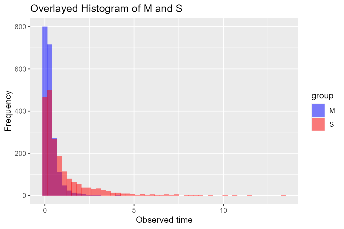

# survival curve by treatment group (A=1 vs. A=0) within strata C1=1
survival_fit_sc <- survfit(Surv(S, ind_S) ~ A, data = sc_data %>% filter(C1==1))
ggsurvplot(survival_fit_sc, data = sc_data, pval = T)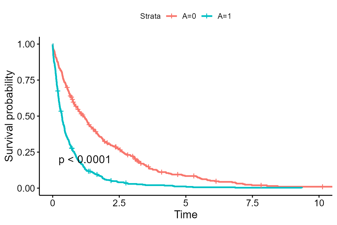

ggsurvplot(survfit(Surv(M, ind_M) ~ A, data = sc_data %>% filter(C1==1)), data = sc_data, pval = T)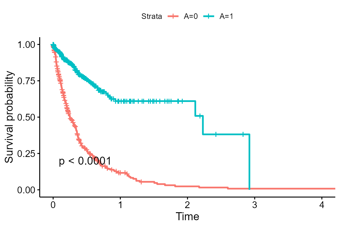

Demonstration

In this setting, we can use a multistate modeling approach to compute the causal estimands of interest (RD, SD, and TE) in the presence of semi-competing risks. We demonstrate how to achieve this using cmest_multistate. In this example, we use the cmest_multistate function to calculate RD and SD for time points 0.1, 0.5, 1, 2, 3, 4, 5, 6. For demonstration purposes, we only run 10 bootstraps here. More number of bootstraps are required in real-world settings (usually >1000). Note this may result in longer computation time. We have implemented parallel computing to speed-up processing time.

# specificy time points (s)
time_to_predict_sc <- c(0.1, 0.5, 1, 2, 3, 4, 5, 6)
# run cmest_multistate()
sc_data_result = cmest_multistate(data = sc_data, 
                                  s = time_to_predict_sc,
                                  multistate_seed = 10,
                                  exposure = 'A', mediator = 'M', outcome = 'S',
                                  yevent = "ind_S",mevent = "ind_M",
                                  basec = c("C1", "C2"),
                                  basecval = c("C1" = "1", 
                                               "C2" = as.character(mean(sc_data$C2))),
                                  astar="0", a="1", 
                                  nboot=10, EMint=F, 
                                  bh_method = "breslow")

The output is a list that consists of 4 elements: 1) The model summary of the joint multistate Cox proportional hazards model fitted on the original dataset, 2) the point estimates of RD and SD for each of the user-specified time points of interest on the original dataset, 3) the summary of the bootstrapped RD, SD, and TE estimates for each of the user-specified time point of interest, including the 2.5%, 50%, and 97.5% percentiles, and 4) the estimated RD, SD, TD for each of the user-specified time point of interest for each bootstrap dataset. These 4 elements of the example output are extracted in order below:

sc_data_result$model_summary

## Call:
## coxph(formula = mstate_form, data = mstate_data_orig, method = bh_method)
## 
##   n= 4823, number of events= 2746 
## 
##          coef exp(coef) se(coef)       z Pr(>|z|)    
## A.1  -1.82713   0.16088  0.09545 -19.143  < 2e-16 ***
## A.2   0.95419   2.59658  0.06776  14.081  < 2e-16 ***
## A.3   0.49085   1.63371  0.10054   4.882 1.05e-06 ***
## M.3  -0.14227   0.86739  0.11808  -1.205  0.22826    
## C1.1  0.07088   1.07346  0.07048   1.006  0.31455    
## C1.2 -0.50335   0.60451  0.06169  -8.160 3.36e-16 ***
## C1.3 -0.18410   0.83185  0.07452  -2.470  0.01349 *  
## C2.1  0.47866   1.61391  0.03507  13.650  < 2e-16 ***
## C2.2  0.29820   1.34743  0.03035   9.824  < 2e-16 ***
## C2.3 -0.11371   0.89252  0.03786  -3.003  0.00267 ** 
## ---
## Signif. codes:  0 '***' 0.001 '**' 0.01 '*' 0.05 '.' 0.1 ' ' 1
## 
##      exp(coef) exp(-coef) lower .95 upper .95
## A.1     0.1609     6.2160    0.1334    0.1940
## A.2     2.5966     0.3851    2.2736    2.9654
## A.3     1.6337     0.6121    1.3415    1.9895
## M.3     0.8674     1.1529    0.6882    1.0933
## C1.1    1.0735     0.9316    0.9350    1.2325
## C1.2    0.6045     1.6542    0.5357    0.6822
## C1.3    0.8319     1.2021    0.7188    0.9627
## C2.1    1.6139     0.6196    1.5067    1.7287
## C2.2    1.3474     0.7422    1.2696    1.4300
## C2.3    0.8925     1.1204    0.8287    0.9613
## 
## Concordance= 0.685  (se = 0.006 )
## Likelihood ratio test= 1088  on 10 df,   p=<2e-16
## Wald test            = 925.2  on 10 df,   p=<2e-16
## Score (logrank) test = 1043  on 10 df,   p=<2e-16

sc_data_result$pt_est

##            RD           SD          TE   s
## 1 -0.10502912 -0.012775776 -0.11780489 0.1
## 2 -0.24042128 -0.102666585 -0.34308786 0.5
## 3 -0.24348137 -0.110141935 -0.35362331 1.0
## 4 -0.19363550 -0.066231071 -0.25986657 2.0
## 5 -0.14446578 -0.033089092 -0.17755487 3.0
## 6 -0.08803151 -0.010953827 -0.09898533 4.0
## 7 -0.06025636 -0.004818455 -0.06507482 5.0
## 8 -0.04331584 -0.002328278 -0.04564411 6.0

sc_data_result$bootstrap_summary

## # A tibble: 8 x 10
##       s RD_median RD_lower RD_higher SD_median SD_lower  SD_higher TE_median
##   <dbl>     <dbl>    <dbl>     <dbl>     <dbl>    <dbl>      <dbl>     <dbl>
## 1   0.1   -0.102   -0.110    -0.0961  -0.0128  -0.0177  -0.00864     -0.116 
## 2   0.5   -0.234   -0.248    -0.218   -0.102   -0.124   -0.0797      -0.335 
## 3   1     -0.237   -0.245    -0.206   -0.109   -0.131   -0.0834      -0.342 
## 4   2     -0.182   -0.199    -0.155   -0.0658  -0.0814  -0.0451      -0.243 
## 5   3     -0.135   -0.152    -0.107   -0.0329  -0.0420  -0.0216      -0.165 
## 6   4     -0.0897  -0.106    -0.0643  -0.0125  -0.0183  -0.00685     -0.0998
## 7   5     -0.0630  -0.0764   -0.0425  -0.00593 -0.0102  -0.00157     -0.0700
## 8   6     -0.0455  -0.0584   -0.0320  -0.00311 -0.00666  0.0000425   -0.0477
## # i 2 more variables: TE_lower <dbl>, TE_higher <dbl>

sc_data_result$raw_output

##             RD            SD          TE   s
## 1  -0.09582917 -0.0107772411 -0.10660642 0.1
## 2  -0.22917879 -0.0956040606 -0.32478285 0.5
## 3  -0.23381887 -0.1061906050 -0.34000947 1.0
## 4  -0.19188951 -0.0721358075 -0.26402532 2.0
## 5  -0.14354416 -0.0361152516 -0.17965941 3.0
## 6  -0.09211269 -0.0133694556 -0.10548214 4.0
## 7  -0.06363802 -0.0060052599 -0.06964328 5.0
## 8  -0.04526898 -0.0028909308 -0.04815991 6.0
## 9  -0.10270269 -0.0101975780 -0.11290027 0.1
## 10 -0.23597628 -0.1118782193 -0.34785450 0.5
## 11 -0.24070013 -0.1167966881 -0.35749682 1.0
## 12 -0.19212659 -0.0727209360 -0.26484753 2.0
## 13 -0.14827707 -0.0394913656 -0.18776843 3.0
## 14 -0.09592120 -0.0150553657 -0.11097657 4.0
## 15 -0.07122535 -0.0079617224 -0.07918707 5.0
## 16 -0.05058930 -0.0038234755 -0.05441277 6.0
## 17 -0.09693900 -0.0112332815 -0.10817228 0.1
## 18 -0.23343985 -0.0982797551 -0.33171960 0.5
## 19 -0.23928404 -0.1102360525 -0.34952009 1.0
## 20 -0.18199828 -0.0580802511 -0.24007854 2.0
## 21 -0.13440543 -0.0282385592 -0.16264399 3.0
## 22 -0.09068223 -0.0117046238 -0.10238685 4.0
## 23 -0.06626005 -0.0058581751 -0.07211823 5.0
## 24 -0.04480515 -0.0024530200 -0.04725817 6.0
## 25 -0.09793323 -0.0145199345 -0.11245317 0.1
## 26 -0.21557079 -0.1072977232 -0.32286852 0.5
## 27 -0.20254389 -0.1205995928 -0.32314349 1.0
## 28 -0.15264324 -0.0719643041 -0.22460755 2.0
## 29 -0.10558425 -0.0340203756 -0.13960462 3.0
## 30 -0.06345066 -0.0128285638 -0.07627922 4.0
## 31 -0.04127673 -0.0057968838 -0.04707362 5.0
## 32 -0.03059641 -0.0033205978 -0.03391701 6.0
## 33 -0.10815761 -0.0180513653 -0.12620898 0.1
## 34 -0.22824872 -0.1274399682 -0.35568869 0.5
## 35 -0.21775347 -0.1320720810 -0.34982555 1.0
## 36 -0.16807077 -0.0817799753 -0.24985074 2.0
## 37 -0.12446830 -0.0427822834 -0.16725059 3.0
## 38 -0.08028276 -0.0174429052 -0.09772566 4.0
## 39 -0.06191568 -0.0104469023 -0.07236258 5.0
## 40 -0.05026881 -0.0069251139 -0.05719392 6.0
## 41 -0.10990960 -0.0081862992 -0.11809590 0.1
## 42 -0.24948467 -0.0751142212 -0.32459890 0.5
## 43 -0.24589034 -0.0781061513 -0.32399649 1.0
## 44 -0.18277687 -0.0428343896 -0.22561126 2.0
## 45 -0.13576508 -0.0205052210 -0.15627030 3.0
## 46 -0.08974293 -0.0063339673 -0.09607690 4.0
## 47 -0.06226701 -0.0011941768 -0.06346118 5.0
## 48 -0.04577031  0.0005167997 -0.04525351 6.0
## 49 -0.10157396 -0.0164019922 -0.11797595 0.1
## 50 -0.22858676 -0.1032477925 -0.33183456 0.5
## 51 -0.24054450 -0.1274389495 -0.36798345 1.0
## 52 -0.20099815 -0.0800934611 -0.28109161 2.0
## 53 -0.15361668 -0.0389193928 -0.19253607 3.0
## 54 -0.10896280 -0.0185782817 -0.12754108 4.0
## 55 -0.07790026 -0.0094570036 -0.08735726 5.0
## 56 -0.06067558 -0.0057602772 -0.06643586 6.0
## 57 -0.10863129 -0.0131850135 -0.12181630 0.1
## 58 -0.23408429 -0.1086367194 -0.34272101 0.5
## 59 -0.22935671 -0.1074535741 -0.33681028 1.0
## 60 -0.16990980 -0.0530827614 -0.22299256 2.0
## 61 -0.12070484 -0.0253251432 -0.14602998 3.0
## 62 -0.07537269 -0.0086399526 -0.08401264 4.0
## 63 -0.04874026 -0.0028788375 -0.05161910 5.0
## 64 -0.03988600 -0.0015910546 -0.04147706 6.0
## 65 -0.10731264 -0.0137684311 -0.12108107 0.1
## 66 -0.24497828 -0.0956314280 -0.34060971 0.5
## 67 -0.24222253 -0.1027302644 -0.34495280 1.0
## 68 -0.18708672 -0.0596861222 -0.24677285 2.0
## 69 -0.14032495 -0.0318100144 -0.17213496 3.0
## 70 -0.08975343 -0.0121777442 -0.10193117 4.0
## 71 -0.06424414 -0.0061427928 -0.07038693 5.0
## 72 -0.04750107 -0.0033241128 -0.05082518 6.0
## 73 -0.10204920 -0.0123379813 -0.11438718 0.1
## 74 -0.23720533 -0.1016881552 -0.33889349 0.5
## 75 -0.22377660 -0.1016116215 -0.32538822 1.0
## 76 -0.16464793 -0.0597299930 -0.22437793 2.0
## 77 -0.11395497 -0.0279571410 -0.14191211 3.0
## 78 -0.06731208 -0.0095785755 -0.07689065 4.0
## 79 -0.04680357 -0.0045775511 -0.05138112 5.0
## 80 -0.03705171 -0.0028278415 -0.03987955 6.0

We here provide an interpretation of RD and SD estimated from this simulated dataset:

TE=x can be interpreted as: The probability of surviving beyond time point s among the exposed group is x higher than that among the unexposed group, controlling for baseline covariates,
RD=x can be interpreted as: The probability of surviving beyond time point s among the exposed group is x higher than that among the unexposed group, controlling for baseline covariates, had the mediator distribution g been the fixed to that of the unexposed group.
SD=x can be interpreted as: The probability of surviving beyond time point s among the exposed group is estimated to increase by x, had the time to mediator distribution among the exposed group been changed to that of the unexposed group, controlling for baseline covariates,

Reference

[1] Valeri, L., Proust-Lima, C., Fan, W., Chen, J. T., & Jacqmin-Gadda, H. (2023). A multistate approach for the study of interventions on an intermediate time-to-event in health disparities research. Statistical Methods in Medical Research, 09622802231163331.

2024-07-01

Data simulation

Demonstration

Reference