Multiple Imputations with Missing Data
2024-07-01
Source:vignettes/multiple_imputation.Rmd
multiple_imputation.RmdThis example demonstrates how to estimate causal effects with
multiple imputations by using cmest when the dataset
contains missing values. For this purpose, we simulate some data
containing a continuous baseline confounder \(C_1\), a binary baseline confounder \(C_2\), a binary exposure \(A\), a binary mediator \(M\) and a binary outcome \(Y\). The true regression models for \(A\), \(M\)
and \(Y\) are: \[logit(E(A|C_1,C_2))=0.2+0.5C_1+0.1C_2\]
\[logit(E(M|A,C_1,C_2))=1+2A+1.5C_1+0.8C_2\]
\[logit(E(Y|A,M,C_1,C_2)))=-3-0.4A-1.2M+0.5AM+0.3C_1-0.6C_2\]
To create the dataset with missing values, we randomly delete 10% of values in the dataset.
set.seed(1)
expit <- function(x) exp(x)/(1+exp(x))
n <- 10000
C1 <- rnorm(n, mean = 1, sd = 0.1)
C2 <- rbinom(n, 1, 0.6)
A <- rbinom(n, 1, expit(0.2 + 0.5*C1 + 0.1*C2))
M <- rbinom(n, 1, expit(1 + 2*A + 1.5*C1 + 0.8*C2))
Y <- rbinom(n, 1, expit(-3 - 0.4*A - 1.2*M + 0.5*A*M + 0.3*C1 - 0.6*C2))
data_noNA <- data.frame(A, M, Y, C1, C2)
missing <- sample(1:(5*n), n*0.1, replace = FALSE)
C1[missing[which(missing <= n)]] <- NA
C2[missing[which((missing > n)*(missing <= 2*n) == 1)] - n] <- NA
A[missing[which((missing > 2*n)*(missing <= 3*n) == 1)] - 2*n] <- NA
M[missing[which((missing > 3*n)*(missing <= 4*n) == 1)] - 3*n] <- NA
Y[missing[which((missing > 4*n)*(missing <= 5*n) == 1)] - 4*n] <- NA
data <- data.frame(A, M, Y, C1, C2)
The DAG for this scientific setting is:
## Registered S3 methods overwritten by 'lme4':
##   method                          from
##   cooks.distance.influence.merMod car
##   influence.merMod                car
##   dfbeta.influence.merMod         car
##   dfbetas.influence.merMod        car
cmdag(outcome = "Y", exposure = "A", mediator = "M",
      basec = c("C1", "C2"), postc = NULL, node = TRUE, text_col = "white")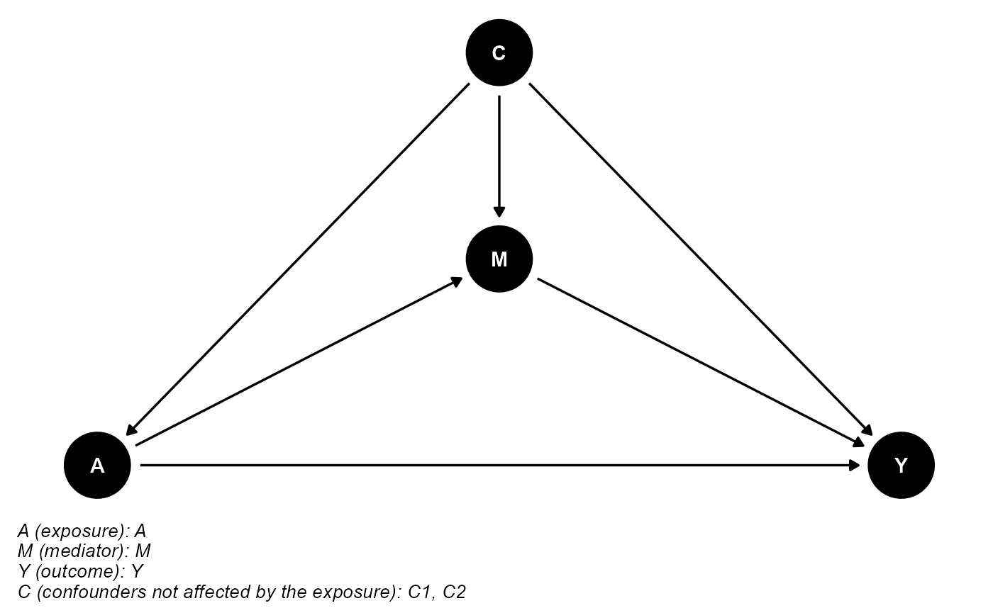
To conduct multiple imputations, we set the multimp
argument to be TRUE. The regression-based approach is used
for illustration. The multiple imputation results:
res_multimp <- cmest(data = data, model = "rb", outcome = "Y", exposure = "A",
                     mediator = "M", basec = c("C1", "C2"), EMint = TRUE,
                     mreg = list("logistic"), yreg = "logistic",
                     astar = 0, a = 1, mval = list(1),
                     estimation = "paramfunc", inference = "delta",
                     multimp = TRUE, args_mice = list(m = 10))
summary(res_multimp)## Causal Mediation Analysis
##
## # Regressions with imputed dataset 1
##
## ## Outcome regression:
##
## Call:
## glm(formula = Y ~ A + M + A * M + C1 + C2, family = binomial(),
## data = getCall(x$reg.output[[1L]]$yreg)$data, weights = getCall(x$reg.output[[1L]]$yreg)$weights)
##
## Deviance Residuals:
## Min 1Q Median 3Q Max
## -0.5560 -0.2416 -0.1755 -0.1615 3.0524
##
## Coefficients:
## Estimate Std. Error z value Pr(>|z|)
## (Intercept) -3.5624 0.7669 -4.645 3.40e-06 ***
## A 0.6413 0.5279 1.215 0.22442
## M -1.0737 0.3738 -2.873 0.00407 **
## C1 0.9419 0.6960 1.353 0.17594
## C2 -0.8335 0.1440 -5.788 7.11e-09 ***
## A:M -0.3402 0.5538 -0.614 0.53897
## ---
## Signif. codes: 0 '***' 0.001 '**' 0.01 '*' 0.05 '.' 0.1 ' ' 1
##
## (Dispersion parameter for binomial family taken to be 1)
##
## Null deviance: 2030.4 on 9999 degrees of freedom
## Residual deviance: 1973.2 on 9994 degrees of freedom
## AIC: 1985.2
##
## Number of Fisher Scoring iterations: 7
##
##
## ## Mediator regressions:
##
## Call:
## glm(formula = M ~ A + C1 + C2, family = binomial(), data = getCall(x$reg.output[[1L]]$mreg[[1L]])$data,
## weights = getCall(x$reg.output[[1L]]$mreg[[1L]])$weights)
##
## Deviance Residuals:
## Min 1Q Median 3Q Max
## -3.2820 0.1137 0.1633 0.2434 0.5946
##
## Coefficients:
## Estimate Std. Error z value Pr(>|z|)
## (Intercept) -0.03518 0.64316 -0.055 0.956376
## A 1.66962 0.14384 11.607 < 2e-16 ***
## C1 2.48028 0.65225 3.803 0.000143 ***
## C2 0.94592 0.13553 6.980 2.96e-12 ***
## ---
## Signif. codes: 0 '***' 0.001 '**' 0.01 '*' 0.05 '.' 0.1 ' ' 1
##
## (Dispersion parameter for binomial family taken to be 1)
##
## Null deviance: 2286.6 on 9999 degrees of freedom
## Residual deviance: 2061.3 on 9996 degrees of freedom
## AIC: 2069.3
##
## Number of Fisher Scoring iterations: 7
##
##
## # Regressions with imputed dataset 2
##
## ## Outcome regression:
##
## Call:
## glm(formula = Y ~ A + M + A * M + C1 + C2, family = binomial(),
## data = getCall(x$reg.output[[2L]]$yreg)$data, weights = getCall(x$reg.output[[2L]]$yreg)$weights)
##
## Deviance Residuals:
## Min 1Q Median 3Q Max
## -0.5540 -0.2437 -0.1701 -0.1590 3.0527
##
## Coefficients:
## Estimate Std. Error z value Pr(>|z|)
## (Intercept) -3.3513 0.7716 -4.343 1.40e-05 ***
## A 0.6633 0.5285 1.255 0.20950
## M -1.0654 0.3738 -2.850 0.00437 **
## C1 0.7414 0.7017 1.057 0.29065
## C2 -0.8794 0.1458 -6.031 1.63e-09 ***
## A:M -0.3846 0.5545 -0.694 0.48788
## ---
## Signif. codes: 0 '***' 0.001 '**' 0.01 '*' 0.05 '.' 0.1 ' ' 1
##
## (Dispersion parameter for binomial family taken to be 1)
##
## Null deviance: 2007.3 on 9999 degrees of freedom
## Residual deviance: 1947.3 on 9994 degrees of freedom
## AIC: 1959.3
##
## Number of Fisher Scoring iterations: 7
##
##
## ## Mediator regressions:
##
## Call:
## glm(formula = M ~ A + C1 + C2, family = binomial(), data = getCall(x$reg.output[[2L]]$mreg[[1L]])$data,
## weights = getCall(x$reg.output[[2L]]$mreg[[1L]])$weights)
##
## Deviance Residuals:
## Min 1Q Median 3Q Max
## -3.2765 0.1127 0.1633 0.2463 0.5698
##
## Coefficients:
## Estimate Std. Error z value Pr(>|z|)
## (Intercept) 0.2522 0.6441 0.392 0.695407
## A 1.7041 0.1453 11.732 < 2e-16 ***
## C1 2.1925 0.6522 3.362 0.000775 ***
## C2 0.9310 0.1358 6.855 7.14e-12 ***
## ---
## Signif. codes: 0 '***' 0.001 '**' 0.01 '*' 0.05 '.' 0.1 ' ' 1
##
## (Dispersion parameter for binomial family taken to be 1)
##
## Null deviance: 2271.9 on 9999 degrees of freedom
## Residual deviance: 2048.6 on 9996 degrees of freedom
## AIC: 2056.6
##
## Number of Fisher Scoring iterations: 7
##
##
## # Regressions with imputed dataset 3
##
## ## Outcome regression:
##
## Call:
## glm(formula = Y ~ A + M + A * M + C1 + C2, family = binomial(),
## data = getCall(x$reg.output[[3L]]$yreg)$data, weights = getCall(x$reg.output[[3L]]$yreg)$weights)
##
## Deviance Residuals:
## Min 1Q Median 3Q Max
## -0.5978 -0.2455 -0.1721 -0.1611 3.0518
##
## Coefficients:
## Estimate Std. Error z value Pr(>|z|)
## (Intercept) -3.3476 0.7664 -4.368 1.25e-05 ***
## A 0.8351 0.5116 1.632 0.10261
## M -1.0600 0.3736 -2.837 0.00455 **
## C1 0.7329 0.6948 1.055 0.29148
## C2 -0.8783 0.1443 -6.085 1.17e-09 ***
## A:M -0.5339 0.5383 -0.992 0.32128
## ---
## Signif. codes: 0 '***' 0.001 '**' 0.01 '*' 0.05 '.' 0.1 ' ' 1
##
## (Dispersion parameter for binomial family taken to be 1)
##
## Null deviance: 2038.1 on 9999 degrees of freedom
## Residual deviance: 1974.0 on 9994 degrees of freedom
## AIC: 1986
##
## Number of Fisher Scoring iterations: 7
##
##
## ## Mediator regressions:
##
## Call:
## glm(formula = M ~ A + C1 + C2, family = binomial(), data = getCall(x$reg.output[[3L]]$mreg[[1L]])$data,
## weights = getCall(x$reg.output[[3L]]$mreg[[1L]])$weights)
##
## Deviance Residuals:
## Min 1Q Median 3Q Max
## -3.2771 0.1135 0.1611 0.2478 0.5803
##
## Coefficients:
## Estimate Std. Error z value Pr(>|z|)
## (Intercept) 0.1175 0.6424 0.183 0.85487
## A 1.7076 0.1451 11.765 < 2e-16 ***
## C1 2.3329 0.6511 3.583 0.00034 ***
## C2 0.9053 0.1351 6.699 2.1e-11 ***
## ---
## Signif. codes: 0 '***' 0.001 '**' 0.01 '*' 0.05 '.' 0.1 ' ' 1
##
## (Dispersion parameter for binomial family taken to be 1)
##
## Null deviance: 2279.3 on 9999 degrees of freedom
## Residual deviance: 2054.9 on 9996 degrees of freedom
## AIC: 2062.9
##
## Number of Fisher Scoring iterations: 7
##
##
## # Regressions with imputed dataset 4
##
## ## Outcome regression:
##
## Call:
## glm(formula = Y ~ A + M + A * M + C1 + C2, family = binomial(),
## data = getCall(x$reg.output[[4L]]$yreg)$data, weights = getCall(x$reg.output[[4L]]$yreg)$weights)
##
## Deviance Residuals:
## Min 1Q Median 3Q Max
## -0.5665 -0.2407 -0.1740 -0.1611 3.0521
##
## Coefficients:
## Estimate Std. Error z value Pr(>|z|)
## (Intercept) -3.3821 0.7635 -4.430 9.42e-06 ***
## A 0.5992 0.5182 1.156 0.247530
## M -1.1938 0.3590 -3.325 0.000884 ***
## C1 0.8605 0.6992 1.231 0.218436
## C2 -0.8218 0.1448 -5.677 1.37e-08 ***
## A:M -0.3001 0.5450 -0.551 0.581866
## ---
## Signif. codes: 0 '***' 0.001 '**' 0.01 '*' 0.05 '.' 0.1 ' ' 1
##
## (Dispersion parameter for binomial family taken to be 1)
##
## Null deviance: 2015.0 on 9999 degrees of freedom
## Residual deviance: 1956.5 on 9994 degrees of freedom
## AIC: 1968.5
##
## Number of Fisher Scoring iterations: 7
##
##
## ## Mediator regressions:
##
## Call:
## glm(formula = M ~ A + C1 + C2, family = binomial(), data = getCall(x$reg.output[[4L]]$mreg[[1L]])$data,
## weights = getCall(x$reg.output[[4L]]$mreg[[1L]])$weights)
##
## Deviance Residuals:
## Min 1Q Median 3Q Max
## -3.2968 0.1106 0.1591 0.2458 0.5925
##
## Coefficients:
## Estimate Std. Error z value Pr(>|z|)
## (Intercept) 0.0239 0.6455 0.037 0.970466
## A 1.7537 0.1466 11.965 < 2e-16 ***
## C1 2.4044 0.6539 3.677 0.000236 ***
## C2 0.9374 0.1359 6.897 5.32e-12 ***
## ---
## Signif. codes: 0 '***' 0.001 '**' 0.01 '*' 0.05 '.' 0.1 ' ' 1
##
## (Dispersion parameter for binomial family taken to be 1)
##
## Null deviance: 2271.9 on 9999 degrees of freedom
## Residual deviance: 2038.1 on 9996 degrees of freedom
## AIC: 2046.1
##
## Number of Fisher Scoring iterations: 7
##
##
## # Regressions with imputed dataset 5
##
## ## Outcome regression:
##
## Call:
## glm(formula = Y ~ A + M + A * M + C1 + C2, family = binomial(),
## data = getCall(x$reg.output[[5L]]$yreg)$data, weights = getCall(x$reg.output[[5L]]$yreg)$weights)
##
## Deviance Residuals:
## Min 1Q Median 3Q Max
## -0.5573 -0.2458 -0.1727 -0.1606 3.0612
##
## Coefficients:
## Estimate Std. Error z value Pr(>|z|)
## (Intercept) -3.2152 0.7541 -4.264 2.01e-05 ***
## A 0.4723 0.5092 0.928 0.353602
## M -1.2817 0.3462 -3.703 0.000213 ***
## C1 0.7980 0.6944 1.149 0.250480
## C2 -0.8747 0.1445 -6.053 1.42e-09 ***
## A:M -0.1467 0.5364 -0.273 0.784508
## ---
## Signif. codes: 0 '***' 0.001 '**' 0.01 '*' 0.05 '.' 0.1 ' ' 1
##
## (Dispersion parameter for binomial family taken to be 1)
##
## Null deviance: 2038.1 on 9999 degrees of freedom
## Residual deviance: 1972.8 on 9994 degrees of freedom
## AIC: 1984.8
##
## Number of Fisher Scoring iterations: 7
##
##
## ## Mediator regressions:
##
## Call:
## glm(formula = M ~ A + C1 + C2, family = binomial(), data = getCall(x$reg.output[[5L]]$mreg[[1L]])$data,
## weights = getCall(x$reg.output[[5L]]$mreg[[1L]])$weights)
##
## Deviance Residuals:
## Min 1Q Median 3Q Max
## -3.2892 0.1105 0.1631 0.2451 0.5819
##
## Coefficients:
## Estimate Std. Error z value Pr(>|z|)
## (Intercept) 0.1842 0.6422 0.287 0.774268
## A 1.7317 0.1457 11.886 < 2e-16 ***
## C1 2.2255 0.6499 3.424 0.000617 ***
## C2 0.9759 0.1358 7.184 6.75e-13 ***
## ---
## Signif. codes: 0 '***' 0.001 '**' 0.01 '*' 0.05 '.' 0.1 ' ' 1
##
## (Dispersion parameter for binomial family taken to be 1)
##
## Null deviance: 2286.6 on 9999 degrees of freedom
## Residual deviance: 2052.2 on 9996 degrees of freedom
## AIC: 2060.2
##
## Number of Fisher Scoring iterations: 7
##
##
## # Regressions with imputed dataset 6
##
## ## Outcome regression:
##
## Call:
## glm(formula = Y ~ A + M + A * M + C1 + C2, family = binomial(),
## data = getCall(x$reg.output[[6L]]$yreg)$data, weights = getCall(x$reg.output[[6L]]$yreg)$weights)
##
## Deviance Residuals:
## Min 1Q Median 3Q Max
## -0.5425 -0.2478 -0.1734 -0.1649 3.0346
##
## Coefficients:
## Estimate Std. Error z value Pr(>|z|)
## (Intercept) -3.0935 0.7581 -4.081 4.49e-05 ***
## A 0.5823 0.5175 1.125 0.2605
## M -1.1526 0.3583 -3.217 0.0013 **
## C1 0.5570 0.6944 0.802 0.4225
## C2 -0.8334 0.1438 -5.796 6.77e-09 ***
## A:M -0.2852 0.5439 -0.524 0.6000
## ---
## Signif. codes: 0 '***' 0.001 '**' 0.01 '*' 0.05 '.' 0.1 ' ' 1
##
## (Dispersion parameter for binomial family taken to be 1)
##
## Null deviance: 2038.1 on 9999 degrees of freedom
## Residual deviance: 1980.0 on 9994 degrees of freedom
## AIC: 1992
##
## Number of Fisher Scoring iterations: 7
##
##
## ## Mediator regressions:
##
## Call:
## glm(formula = M ~ A + C1 + C2, family = binomial(), data = getCall(x$reg.output[[6L]]$mreg[[1L]])$data,
## weights = getCall(x$reg.output[[6L]]$mreg[[1L]])$weights)
##
## Deviance Residuals:
## Min 1Q Median 3Q Max
## -3.2831 0.1116 0.1635 0.2465 0.5820
##
## Coefficients:
## Estimate Std. Error z value Pr(>|z|)
## (Intercept) 0.1784 0.6435 0.277 0.781575
## A 1.7256 0.1449 11.906 < 2e-16 ***
## C1 2.2335 0.6511 3.430 0.000603 ***
## C2 0.9586 0.1354 7.081 1.44e-12 ***
## ---
## Signif. codes: 0 '***' 0.001 '**' 0.01 '*' 0.05 '.' 0.1 ' ' 1
##
## (Dispersion parameter for binomial family taken to be 1)
##
## Null deviance: 2294.0 on 9999 degrees of freedom
## Residual deviance: 2061.5 on 9996 degrees of freedom
## AIC: 2069.5
##
## Number of Fisher Scoring iterations: 7
##
##
## # Regressions with imputed dataset 7
##
## ## Outcome regression:
##
## Call:
## glm(formula = Y ~ A + M + A * M + C1 + C2, family = binomial(),
## data = getCall(x$reg.output[[7L]]$yreg)$data, weights = getCall(x$reg.output[[7L]]$yreg)$weights)
##
## Deviance Residuals:
## Min 1Q Median 3Q Max
## -0.5639 -0.2415 -0.1744 -0.1606 3.0539
##
## Coefficients:
## Estimate Std. Error z value Pr(>|z|)
## (Intercept) -3.5496 0.7698 -4.611 4.01e-06 ***
## A 0.6739 0.5284 1.275 0.20215
## M -1.0735 0.3738 -2.872 0.00408 **
## C1 0.9293 0.6985 1.330 0.18336
## C2 -0.8402 0.1445 -5.815 6.07e-09 ***
## A:M -0.3776 0.5543 -0.681 0.49573
## ---
## Signif. codes: 0 '***' 0.001 '**' 0.01 '*' 0.05 '.' 0.1 ' ' 1
##
## (Dispersion parameter for binomial family taken to be 1)
##
## Null deviance: 2022.7 on 9999 degrees of freedom
## Residual deviance: 1964.8 on 9994 degrees of freedom
## AIC: 1976.8
##
## Number of Fisher Scoring iterations: 7
##
##
## ## Mediator regressions:
##
## Call:
## glm(formula = M ~ A + C1 + C2, family = binomial(), data = getCall(x$reg.output[[7L]]$mreg[[1L]])$data,
## weights = getCall(x$reg.output[[7L]]$mreg[[1L]])$weights)
##
## Deviance Residuals:
## Min 1Q Median 3Q Max
## -3.2951 0.1118 0.1615 0.2428 0.5994
##
## Coefficients:
## Estimate Std. Error z value Pr(>|z|)
## (Intercept) -0.08708 0.64471 -0.135 0.892561
## A 1.70024 0.14529 11.702 < 2e-16 ***
## C1 2.53093 0.65396 3.870 0.000109 ***
## C2 0.95308 0.13616 7.000 2.56e-12 ***
## ---
## Signif. codes: 0 '***' 0.001 '**' 0.01 '*' 0.05 '.' 0.1 ' ' 1
##
## (Dispersion parameter for binomial family taken to be 1)
##
## Null deviance: 2271.9 on 9999 degrees of freedom
## Residual deviance: 2043.1 on 9996 degrees of freedom
## AIC: 2051.1
##
## Number of Fisher Scoring iterations: 7
##
##
## # Regressions with imputed dataset 8
##
## ## Outcome regression:
##
## Call:
## glm(formula = Y ~ A + M + A * M + C1 + C2, family = binomial(),
## data = getCall(x$reg.output[[8L]]$yreg)$data, weights = getCall(x$reg.output[[8L]]$yreg)$weights)
##
## Deviance Residuals:
## Min 1Q Median 3Q Max
## -0.5742 -0.2415 -0.1753 -0.1619 3.0350
##
## Coefficients:
## Estimate Std. Error z value Pr(>|z|)
## (Intercept) -3.5985 0.7640 -4.710 2.48e-06 ***
## A 0.7253 0.5288 1.372 0.1702
## M -1.0158 0.3725 -2.727 0.0064 **
## C1 0.9601 0.6929 1.385 0.1659
## C2 -0.8179 0.1434 -5.703 1.18e-08 ***
## A:M -0.4815 0.5539 -0.869 0.3847
## ---
## Signif. codes: 0 '***' 0.001 '**' 0.01 '*' 0.05 '.' 0.1 ' ' 1
##
## (Dispersion parameter for binomial family taken to be 1)
##
## Null deviance: 2038.1 on 9999 degrees of freedom
## Residual deviance: 1982.5 on 9994 degrees of freedom
## AIC: 1994.5
##
## Number of Fisher Scoring iterations: 7
##
##
## ## Mediator regressions:
##
## Call:
## glm(formula = M ~ A + C1 + C2, family = binomial(), data = getCall(x$reg.output[[8L]]$mreg[[1L]])$data,
## weights = getCall(x$reg.output[[8L]]$mreg[[1L]])$weights)
##
## Deviance Residuals:
## Min 1Q Median 3Q Max
## -3.2971 0.1107 0.1584 0.2465 0.5975
##
## Coefficients:
## Estimate Std. Error z value Pr(>|z|)
## (Intercept) -0.02998 0.64194 -0.047 0.962749
## A 1.75748 0.14646 11.999 < 2e-16 ***
## C1 2.45664 0.65105 3.773 0.000161 ***
## C2 0.92943 0.13550 6.859 6.91e-12 ***
## ---
## Signif. codes: 0 '***' 0.001 '**' 0.01 '*' 0.05 '.' 0.1 ' ' 1
##
## (Dispersion parameter for binomial family taken to be 1)
##
## Null deviance: 2279.3 on 9999 degrees of freedom
## Residual deviance: 2043.4 on 9996 degrees of freedom
## AIC: 2051.4
##
## Number of Fisher Scoring iterations: 7
##
##
## # Regressions with imputed dataset 9
##
## ## Outcome regression:
##
## Call:
## glm(formula = Y ~ A + M + A * M + C1 + C2, family = binomial(),
## data = getCall(x$reg.output[[9L]]$yreg)$data, weights = getCall(x$reg.output[[9L]]$yreg)$weights)
##
## Deviance Residuals:
## Min 1Q Median 3Q Max
## -0.5625 -0.2385 -0.1746 -0.1606 3.0559
##
## Coefficients:
## Estimate Std. Error z value Pr(>|z|)
## (Intercept) -3.5868 0.7729 -4.641 3.47e-06 ***
## A 0.6867 0.5282 1.300 0.19357
## M -1.0834 0.3741 -2.896 0.00378 **
## C1 0.9452 0.7020 1.346 0.17818
## C2 -0.8130 0.1452 -5.600 2.15e-08 ***
## A:M -0.3861 0.5546 -0.696 0.48624
## ---
## Signif. codes: 0 '***' 0.001 '**' 0.01 '*' 0.05 '.' 0.1 ' ' 1
##
## (Dispersion parameter for binomial family taken to be 1)
##
## Null deviance: 1999.6 on 9999 degrees of freedom
## Residual deviance: 1944.1 on 9994 degrees of freedom
## AIC: 1956.1
##
## Number of Fisher Scoring iterations: 7
##
##
## ## Mediator regressions:
##
## Call:
## glm(formula = M ~ A + C1 + C2, family = binomial(), data = getCall(x$reg.output[[9L]]$mreg[[1L]])$data,
## weights = getCall(x$reg.output[[9L]]$mreg[[1L]])$weights)
##
## Deviance Residuals:
## Min 1Q Median 3Q Max
## -3.2818 0.1126 0.1620 0.2472 0.5857
##
## Coefficients:
## Estimate Std. Error z value Pr(>|z|)
## (Intercept) 0.09774 0.64135 0.152 0.878874
## A 1.71875 0.14492 11.860 < 2e-16 ***
## C1 2.33198 0.64966 3.590 0.000331 ***
## C2 0.93071 0.13509 6.889 5.6e-12 ***
## ---
## Signif. codes: 0 '***' 0.001 '**' 0.01 '*' 0.05 '.' 0.1 ' ' 1
##
## (Dispersion parameter for binomial family taken to be 1)
##
## Null deviance: 2294.0 on 9999 degrees of freedom
## Residual deviance: 2063.6 on 9996 degrees of freedom
## AIC: 2071.6
##
## Number of Fisher Scoring iterations: 7
##
##
## # Regressions with imputed dataset 10
##
## ## Outcome regression:
##
## Call:
## glm(formula = Y ~ A + M + A * M + C1 + C2, family = binomial(),
## data = getCall(x$reg.output[[10L]]$yreg)$data, weights = getCall(x$reg.output[[10L]]$yreg)$weights)
##
## Deviance Residuals:
## Min 1Q Median 3Q Max
## -0.6006 -0.2466 -0.1696 -0.1596 3.0471
##
## Coefficients:
## Estimate Std. Error z value Pr(>|z|)
## (Intercept) -3.2053 0.7595 -4.220 2.44e-05 ***
## A 0.7631 0.5012 1.523 0.12786
## M -1.1229 0.3580 -3.137 0.00171 **
## C1 0.6827 0.6961 0.981 0.32674
## C2 -0.8995 0.1449 -6.210 5.31e-10 ***
## A:M -0.4937 0.5281 -0.935 0.34987
## ---
## Signif. codes: 0 '***' 0.001 '**' 0.01 '*' 0.05 '.' 0.1 ' ' 1
##
## (Dispersion parameter for binomial family taken to be 1)
##
## Null deviance: 2038.1 on 9999 degrees of freedom
## Residual deviance: 1970.7 on 9994 degrees of freedom
## AIC: 1982.7
##
## Number of Fisher Scoring iterations: 7
##
##
## ## Mediator regressions:
##
## Call:
## glm(formula = M ~ A + C1 + C2, family = binomial(), data = getCall(x$reg.output[[10L]]$mreg[[1L]])$data,
## weights = getCall(x$reg.output[[10L]]$mreg[[1L]])$weights)
##
## Deviance Residuals:
## Min 1Q Median 3Q Max
## -3.3026 0.1094 0.1600 0.2428 0.5976
##
## Coefficients:
## Estimate Std. Error z value Pr(>|z|)
## (Intercept) 0.003158 0.643227 0.005 0.996083
## A 1.745766 0.146506 11.916 < 2e-16 ***
## C1 2.407423 0.652168 3.691 0.000223 ***
## C2 0.981818 0.136344 7.201 5.98e-13 ***
## ---
## Signif. codes: 0 '***' 0.001 '**' 0.01 '*' 0.05 '.' 0.1 ' ' 1
##
## (Dispersion parameter for binomial family taken to be 1)
##
## Null deviance: 2279.3 on 9999 degrees of freedom
## Residual deviance: 2039.5 on 9996 degrees of freedom
## AIC: 2047.5
##
## Number of Fisher Scoring iterations: 7
##
##
## # Effect decomposition on the odds ratio scale via the regression-based approach with multiple imputation
##
## Closed-form parameter function estimation with
## delta method standard errors, confidence intervals and p-values
##
## Estimate Std.error 95% CIL 95% CIU P.val
## Rcde 1.33818 0.22617 0.96084 1.864 0.0848 .
## Rpnde 1.41766 0.23702 1.02154 1.967 0.0368 *
## Rtnde 1.35411 0.22314 0.98036 1.870 0.0658 .
## Rpnie 0.92797 0.03740 0.85750 1.004 0.0636 .
## Rtnie 0.88638 0.05341 0.78763 0.998 0.0453 *
## Rte 1.25658 0.19851 0.92198 1.713 0.1482
## ERcde 0.30838 0.20145 -0.08645 0.703 0.1258
## ERintref 0.10948 0.11563 -0.11715 0.336 0.3437
## ERintmed -0.08911 0.09429 -0.27392 0.096 0.3446
## ERpnie -0.07199 0.03736 -0.14522 0.001 0.0540 .
## ERcde(prop) 1.20207 0.26051 0.69148 1.713 3.94e-06 ***
## ERintref(prop) 0.43032 0.50804 -0.56542 1.426 0.3970
## ERintmed(prop) -0.35041 0.41505 -1.16389 0.463 0.3985
## ERpnie(prop) -0.28198 0.26120 -0.79394 0.230 0.2803
## pm -0.63239 0.53431 -1.67962 0.415 0.2366
## int 0.07991 0.09394 -0.10421 0.264 0.3950
## pe -0.20207 0.26051 -0.71267 0.309 0.4379
## ---
## Signif. codes: 0 '***' 0.001 '**' 0.01 '*' 0.05 '.' 0.1 ' ' 1
##
## (Rcde: controlled direct effect odds ratio; Rpnde: pure natural direct effect odds ratio; Rtnde: total natural direct effect odds ratio; Rpnie: pure natural indirect effect odds ratio; Rtnie: total natural indirect effect odds ratio; Rte: total effect odds ratio; ERcde: excess relative risk due to controlled direct effect; ERintref: excess relative risk due to reference interaction; ERintmed: excess relative risk due to mediated interaction; ERpnie: excess relative risk due to pure natural indirect effect; ERcde(prop): proportion ERcde; ERintref(prop): proportion ERintref; ERintmed(prop): proportion ERintmed; ERpnie(prop): proportion ERpnie; pm: overall proportion mediated; int: overall proportion attributable to interaction; pe: overall proportion eliminated)
##
## Relevant variable values:
## $a
## [1] 1
##
## $astar
## [1] 0
##
## $yval
## [1] "1"
##
## $mval
## $mval[[1]]
## [1] 1
##
##
## $basecval
## $basecval[[1]]
## [1] 0.9993387
##
## $basecval[[2]]
## [1] 0.6060235Compare the multiple imputation results with true results:
res_noNA <- cmest(data = data_noNA, model = "rb", outcome = "Y", exposure = "A",
                  mediator = "M", basec = c("C1", "C2"), EMint = TRUE,
                  mreg = list("logistic"), yreg = "logistic",
                  astar = 0, a = 1, mval = list(1),
                  estimation = "paramfunc", inference = "delta")
summary(res_noNA)## Causal Mediation Analysis
##
## # Outcome regression:
##
## Call:
## glm(formula = Y ~ A + M + A * M + C1 + C2, family = binomial(),
## data = getCall(x$reg.output$yreg)$data, weights = getCall(x$reg.output$yreg)$weights)
##
## Deviance Residuals:
## Min 1Q Median 3Q Max
## -0.5681 -0.2414 -0.1741 -0.1604 3.0521
##
## Coefficients:
## Estimate Std. Error z value Pr(>|z|)
## (Intercept) -3.5731 0.7713 -4.633 3.61e-06 ***
## A 0.7084 0.5283 1.341 0.17990
## M -1.0471 0.3736 -2.803 0.00507 **
## C1 0.9337 0.6973 1.339 0.18054
## C2 -0.8415 0.1443 -5.829 5.56e-09 ***
## A:M -0.4222 0.5541 -0.762 0.44607
## ---
## Signif. codes: 0 '***' 0.001 '**' 0.01 '*' 0.05 '.' 0.1 ' ' 1
##
## (Dispersion parameter for binomial family taken to be 1)
##
## Null deviance: 2022.7 on 9999 degrees of freedom
## Residual deviance: 1965.0 on 9994 degrees of freedom
## AIC: 1977
##
## Number of Fisher Scoring iterations: 7
##
##
## # Mediator regressions:
##
## Call:
## glm(formula = M ~ A + C1 + C2, family = binomial(), data = getCall(x$reg.output$mreg[[1L]])$data,
## weights = getCall(x$reg.output$mreg[[1L]])$weights)
##
## Deviance Residuals:
## Min 1Q Median 3Q Max
## -3.2578 0.1145 0.1647 0.2519 0.5563
##
## Coefficients:
## Estimate Std. Error z value Pr(>|z|)
## (Intercept) 0.4353 0.6410 0.679 0.49712
## A 1.7076 0.1443 11.837 < 2e-16 ***
## C1 1.9982 0.6474 3.086 0.00203 **
## C2 0.9024 0.1345 6.709 1.96e-11 ***
## ---
## Signif. codes: 0 '***' 0.001 '**' 0.01 '*' 0.05 '.' 0.1 ' ' 1
##
## (Dispersion parameter for binomial family taken to be 1)
##
## Null deviance: 2294.0 on 9999 degrees of freedom
## Residual deviance: 2072.5 on 9996 degrees of freedom
## AIC: 2080.5
##
## Number of Fisher Scoring iterations: 7
##
##
## # Effect decomposition on the odds ratio scale via the regression-based approach
##
## Closed-form parameter function estimation with
## delta method standard errors, confidence intervals and p-values
##
## Estimate Std.error 95% CIL 95% CIU P.val
## Rcde 1.33138 0.22278 0.95912 1.848 0.0872 .
## Rpnde 1.41988 0.23708 1.02358 1.970 0.0358 *
## Rtnde 1.34928 0.22056 0.97940 1.859 0.0669 .
## Rpnie 0.93338 0.03576 0.86587 1.006 0.0719 .
## Rtnie 0.88697 0.05295 0.78902 0.997 0.0445 *
## Rte 1.25939 0.19804 0.92535 1.714 0.1425
## ERcde 0.30416 0.20019 -0.08820 0.697 0.1287
## ERintref 0.11571 0.11472 -0.10914 0.341 0.3131
## ERintmed -0.09387 0.09323 -0.27659 0.089 0.3140
## ERpnie -0.06662 0.03576 -0.13670 0.003 0.0624 .
## ERcde(prop) 1.17262 0.23540 0.71124 1.634 6.32e-07 ***
## ERintref(prop) 0.44610 0.49051 -0.51528 1.407 0.3631
## ERintmed(prop) -0.36189 0.39881 -1.14354 0.420 0.3642
## ERpnie(prop) -0.25684 0.23474 -0.71691 0.203 0.2739
## pm -0.61872 0.50289 -1.60437 0.367 0.2186
## int 0.08421 0.09264 -0.09736 0.266 0.3633
## pe -0.17262 0.23540 -0.63400 0.289 0.4634
## ---
## Signif. codes: 0 '***' 0.001 '**' 0.01 '*' 0.05 '.' 0.1 ' ' 1
##
## (Rcde: controlled direct effect odds ratio; Rpnde: pure natural direct effect odds ratio; Rtnde: total natural direct effect odds ratio; Rpnie: pure natural indirect effect odds ratio; Rtnie: total natural indirect effect odds ratio; Rte: total effect odds ratio; ERcde: excess relative risk due to controlled direct effect; ERintref: excess relative risk due to reference interaction; ERintmed: excess relative risk due to mediated interaction; ERpnie: excess relative risk due to pure natural indirect effect; ERcde(prop): proportion ERcde; ERintref(prop): proportion ERintref; ERintmed(prop): proportion ERintmed; ERpnie(prop): proportion ERpnie; pm: overall proportion mediated; int: overall proportion attributable to interaction; pe: overall proportion eliminated)
##
## Relevant variable values:
## $a
## [1] 1
##
## $astar
## [1] 0
##
## $yval
## [1] "1"
##
## $mval
## $mval[[1]]
## [1] 1
##
##
## $basecval
## $basecval[[1]]
## [1] 0.9993463
##
## $basecval[[2]]
## [1] 0.6061