We illustrate the general workflow of the CMAverse
package by a quick example. The general workflow is:
Plot the DAG of causal relationships using
cmdag.Estimate causal effects and make inferences using
cmest.Conduct sensitivity analysis for unmeasured confounding and measurement error using
cmsens.
Firstly, let’s load the package.
## Registered S3 methods overwritten by 'lme4':
##   method                          from
##   cooks.distance.influence.merMod car
##   influence.merMod                car
##   dfbeta.influence.merMod         car
##   dfbetas.influence.merMod        car
Next, we simulate some data and plot the DAG. The simulated dataset contains a binary exposure, a binary mediator, a continuous mediator, a continuous outcome and two baseline confounders.
set.seed(1)
n <- 100
C1 <- rnorm(n, mean = 1, sd = 1)
C2 <- rbinom(n, 1, 0.6)
pa <- exp(0.2 - 0.5*C1 + 0.1*C2)/(1 + exp(0.2 - 0.5*C1 + 0.1*C2))
A <- rbinom(n, 1, pa)
pm <- exp(1 + 0.5*A - 1.5*C1 + 0.5*C2)/ (1 + exp(1 + 0.5*A - 1.5*C1 + 0.5*C2))
M1 <- rbinom(n, 1, pm)
M2 <- rnorm(n, 2 + 0.8*A - M1 + 0.5*C1 + 2*C2, 1)
Y <- rnorm(n, mean = 0.5 + 0.4*A + 0.5*M1 + 0.6*M2 + 0.3*A*M1 + 0.2*A*M2 - 0.3*C1 + 2*C2, sd = 1)
data <- data.frame(A, M1, M2, Y, C1, C2)
The DAG can be plotted using cmdag.
cmdag(outcome = "Y", exposure = "A", mediator = c("M1", "M2"),
      basec = c("C1", "C2"), postc = NULL, node = FALSE, text_col = "black")
Then, we estimate causal effects using cmest. We use the
regression-based approach for illustration. The reference values for the
exposure are set to be 0 and 1. The reference values for the two
mediators are set to be 1.
est <- cmest(data = data, model = "rb", outcome = "Y", exposure = "A",
                mediator = c("M1", "M2"), basec = c("C1", "C2"), EMint = TRUE,
                mreg = list("logistic", "linear"), yreg = "linear",
                astar = 0, a = 1, mval = list(1, 1),
                estimation = "imputation", inference = "bootstrap", nboot = 20)
Summarize and plot the results:
summary(est)## Causal Mediation Analysis
##
## # Outcome regression:
##
## Call:
## glm(formula = Y ~ A + M1 + M2 + A * M1 + A * M2 + C1 + C2, family = gaussian(),
## data = getCall(x$reg.output$yreg)$data, weights = getCall(x$reg.output$yreg)$weights)
##
## Deviance Residuals:
## Min 1Q Median 3Q Max
## -2.47763 -0.59177 0.03214 0.66470 1.92837
##
## Coefficients:
## Estimate Std. Error t value Pr(>|t|)
## (Intercept) -0.429317 0.446678 -0.961 0.3390
## A 1.305199 0.751816 1.736 0.0859 .
## M1 0.762169 0.310811 2.452 0.0161 *
## M2 0.691868 0.132038 5.240 1.01e-06 ***
## C1 -0.197350 0.136885 -1.442 0.1528
## C2 2.389790 0.355404 6.724 1.46e-09 ***
## A:M1 0.127853 0.466496 0.274 0.7846
## A:M2 -0.001608 0.151163 -0.011 0.9915
## ---
## Signif. codes: 0 '***' 0.001 '**' 0.01 '*' 0.05 '.' 0.1 ' ' 1
##
## (Dispersion parameter for gaussian family taken to be 1.100923)
##
## Null deviance: 571.51 on 99 degrees of freedom
## Residual deviance: 101.28 on 92 degrees of freedom
## AIC: 303.06
##
## Number of Fisher Scoring iterations: 2
##
##
## # Mediator regressions:
##
## Call:
## glm(formula = M1 ~ A + C1 + C2, family = binomial(), data = getCall(x$reg.output$mreg[[1L]])$data,
## weights = getCall(x$reg.output$mreg[[1L]])$weights)
##
## Deviance Residuals:
## Min 1Q Median 3Q Max
## -1.9623 -0.9462 -0.4322 0.9679 2.2586
##
## Coefficients:
## Estimate Std. Error z value Pr(>|z|)
## (Intercept) 0.003446 0.547959 0.006 0.994982
## A 0.828694 0.456732 1.814 0.069616 .
## C1 -0.984454 0.292880 -3.361 0.000776 ***
## C2 0.892199 0.511832 1.743 0.081308 .
## ---
## Signif. codes: 0 '***' 0.001 '**' 0.01 '*' 0.05 '.' 0.1 ' ' 1
##
## (Dispersion parameter for binomial family taken to be 1)
##
## Null deviance: 138.47 on 99 degrees of freedom
## Residual deviance: 115.67 on 96 degrees of freedom
## AIC: 123.67
##
## Number of Fisher Scoring iterations: 3
##
##
##
## Call:
## glm(formula = M2 ~ A + C1 + C2, family = gaussian(), data = getCall(x$reg.output$mreg[[2L]])$data,
## weights = getCall(x$reg.output$mreg[[2L]])$weights)
##
## Deviance Residuals:
## Min 1Q Median 3Q Max
## -2.60482 -0.60844 0.02378 0.58801 2.59561
##
## Coefficients:
## Estimate Std. Error t value Pr(>|t|)
## (Intercept) 1.6403 0.2564 6.397 5.75e-09 ***
## A 0.2901 0.2170 1.337 0.184
## C1 0.6208 0.1189 5.219 1.04e-06 ***
## C2 2.0833 0.2366 8.806 5.44e-14 ***
## ---
## Signif. codes: 0 '***' 0.001 '**' 0.01 '*' 0.05 '.' 0.1 ' ' 1
##
## (Dispersion parameter for gaussian family taken to be 1.110528)
##
## Null deviance: 225.08 on 99 degrees of freedom
## Residual deviance: 106.61 on 96 degrees of freedom
## AIC: 300.19
##
## Number of Fisher Scoring iterations: 2
##
##
## # Effect decomposition on the mean difference scale via the regression-based approach
##
## Direct counterfactual imputation estimation with
## bootstrap standard errors, percentile confidence intervals and p-values
##
## Estimate Std.error 95% CIL 95% CIU P.val
## cde 1.431445 0.406563 0.791552 2.177 <2e-16 ***
## pnde 1.345009 0.210568 1.034657 1.751 <2e-16 ***
## tnde 1.363720 0.222721 1.001818 1.727 <2e-16 ***
## pnie 0.315062 0.175113 0.012484 0.526 0.1 .
## tnie 0.333773 0.150220 0.011253 0.510 <2e-16 ***
## te 1.678782 0.282291 1.201192 2.157 <2e-16 ***
## intref -0.086436 0.340713 -0.716350 0.427 0.7
## intmed 0.018712 0.094136 -0.148749 0.177 1.0
## cde(prop) 0.852669 0.204465 0.517111 1.231 <2e-16 ***
## intref(prop) -0.051487 0.223188 -0.496311 0.279 0.7
## intmed(prop) 0.011146 0.054510 -0.083948 0.103 1.0
## pnie(prop) 0.187673 0.099768 0.009682 0.317 0.1 .
## pm 0.198819 0.084045 0.008982 0.292 <2e-16 ***
## int -0.040341 0.234302 -0.528828 0.273 0.7
## pe 0.147331 0.204465 -0.230814 0.483 0.6
## ---
## Signif. codes: 0 '***' 0.001 '**' 0.01 '*' 0.05 '.' 0.1 ' ' 1
##
## (cde: controlled direct effect; pnde: pure natural direct effect; tnde: total natural direct effect; pnie: pure natural indirect effect; tnie: total natural indirect effect; te: total effect; intref: reference interaction; intmed: mediated interaction; cde(prop): proportion cde; intref(prop): proportion intref; intmed(prop): proportion intmed; pnie(prop): proportion pnie; pm: overall proportion mediated; int: overall proportion attributable to interaction; pe: overall proportion eliminated)
##
## Relevant variable values:
## $a
## [1] 1
##
## $astar
## [1] 0
##
## $mval
## $mval[[1]]
## [1] 1
##
## $mval[[2]]
## [1] 1
ggcmest(est) +
  ggplot2::theme(axis.text.x = ggplot2::element_text(angle = 30, vjust = 0.8))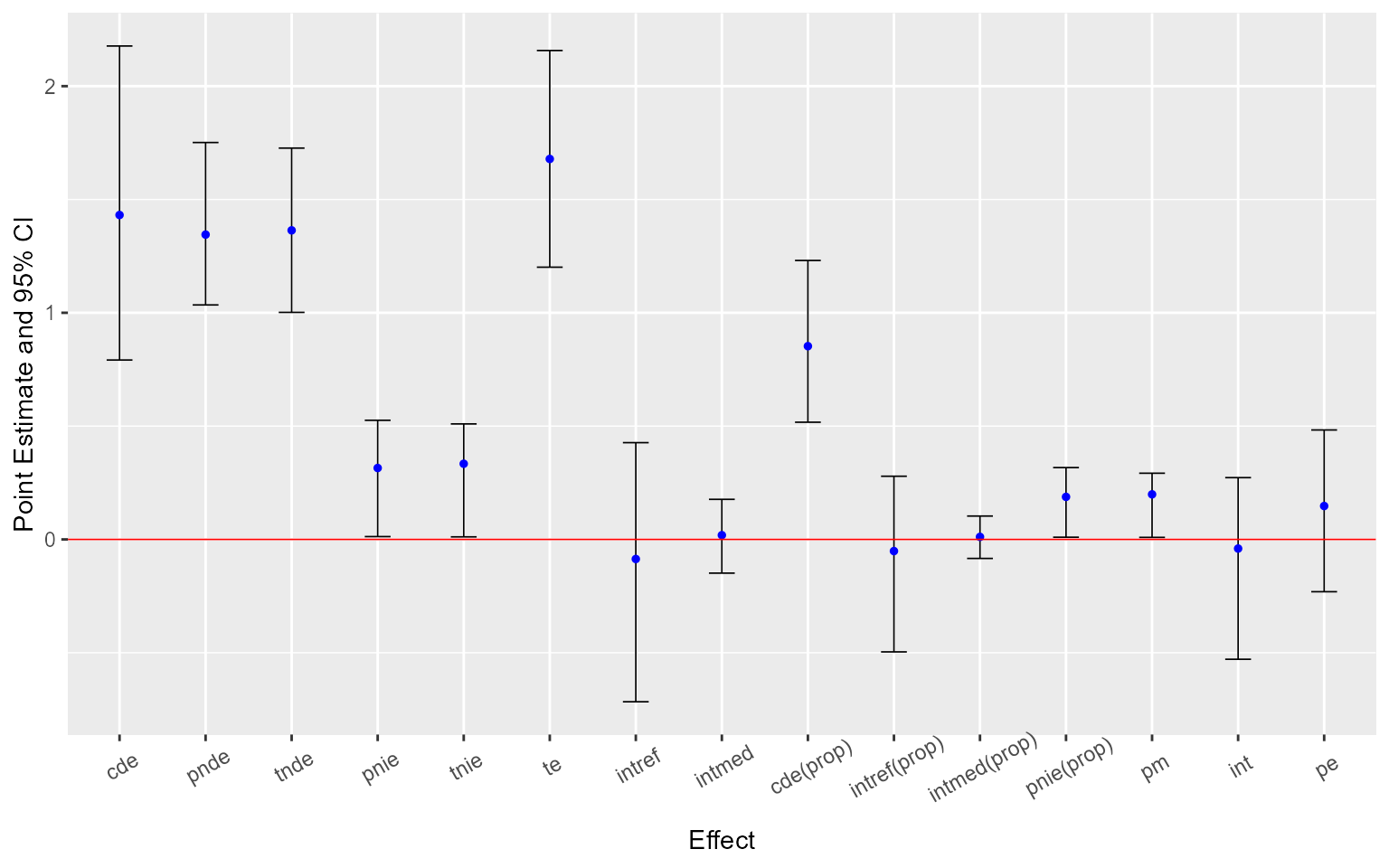
Lastly, we conduct sensitivity analysis for the results. Sensitivity analysis for unmeasured confounding:
cmsens(object = est, sens = "uc")## Sensitivity Analysis For Unmeasured Confounding
##
## Evalues on the risk or rate ratio scale:
## estRR lowerRR upperRR Evalue.estRR Evalue.lowerRR Evalue.upperRR
## cde 1.719704 1.2724617 2.324143 2.832214 1.861272 NA
## pnde 1.664318 1.4239257 1.945293 2.715810 2.200868 NA
## tnde 1.676154 1.4211994 1.976847 2.740738 2.194897 NA
## pnie 1.126739 0.9896507 1.282818 1.504631 1.000000 NA
## tnie 1.134753 1.0152410 1.268333 1.525791 1.139632 NA
## te 1.888589 1.5321886 2.327891 3.184035 2.435191 NAAssume that \(C_1\) was measured with error. Sensitivity analysis for measurement error using regression calibration with a set of assumed error standard deviations 0.1, 0.2 and 0.3:
me1 <- cmsens(object = est, sens = "me", MEmethod = "rc",
              MEvariable = "C1", MEvartype = "con", MEerror = c(0.1, 0.2, 0.3))
Summarize and plot the results:
summary(me1)## Sensitivity Analysis For Measurement Error
##
## The variable measured with error: C1
## Type of the variable measured with error: continuous
##
## # Measurement error 1:
## [1] 0.1
##
## ## Error-corrected regressions for measurement error 1:
##
## ### Outcome regression:
## Call:
## rcreg(reg = getCall(x$sens[[1L]]$reg.output$yreg)$reg, formula = Y ~
## A + M1 + M2 + A * M1 + A * M2 + C1 + C2, data = getCall(x$sens[[1L]]$reg.output$yreg)$data,
## MEvariable = "C1", MEerror = 0.1, variance = TRUE, nboot = 400,
## weights = getCall(x$sens[[1L]]$reg.output$yreg)$weights)
##
## Naive coefficient estimates:
## (Intercept) A M1 M2 C1 C2
## -0.429317055 1.305199111 0.762169424 0.691868043 -0.197349688 2.389790272
## A:M1 A:M2
## 0.127853354 -0.001607689
##
## Naive var-cov estimates:
## (Intercept) A M1 M2 C1
## (Intercept) 0.19952129 -0.186177297 -0.071800151 -0.042143887 -0.012473494
## A -0.18617730 0.565227608 0.061763824 0.035566831 0.008550886
## M1 -0.07180015 0.061763824 0.096603550 0.011127995 0.008367323
## M2 -0.04214389 0.035566831 0.011127995 0.017433949 -0.005541985
## C1 -0.01247349 0.008550886 0.008367323 -0.005541985 0.018737581
## C2 0.03202116 -0.002076496 -0.025485517 -0.031937394 0.011413789
## A:M1 0.05250394 -0.194186113 -0.081844376 0.001218548 -0.006350845
## A:M2 0.03868322 -0.102112096 -0.008061219 -0.010381316 -0.000334026
## C2 A:M1 A:M2
## (Intercept) 0.032021156 0.052503937 0.038683218
## A -0.002076496 -0.194186113 -0.102112096
## M1 -0.025485517 -0.081844376 -0.008061219
## M2 -0.031937394 0.001218548 -0.010381316
## C1 0.011413789 -0.006350845 -0.000334026
## C2 0.126311866 -0.027375016 0.006147880
## A:M1 -0.027375016 0.217618968 0.019236723
## A:M2 0.006147880 0.019236723 0.022850334
##
## Variable measured with error:
## C1
## Measurement error:
## 0.1
## Error-corrected results:
## Estimate Std. Error t value Pr(>|t|)
## (Intercept) -0.427276 0.491050 -0.870 0.3865
## A 1.304514 0.698672 1.867 0.0651 .
## M1 0.761089 0.367873 2.069 0.0414 *
## M2 0.692841 0.138823 4.991 2.83e-06 ***
## C1 -0.200697 0.125629 -1.598 0.1136
## C2 2.387891 0.403462 5.919 5.52e-08 ***
## A:M1 0.127853 0.419520 0.305 0.7612
## A:M2 -0.001608 0.146484 -0.011 0.9913
## ---
## Signif. codes: 0 '***' 0.001 '**' 0.01 '*' 0.05 '.' 0.1 ' ' 1
##
## ### Mediator regressions:
## Call:
## rcreg(reg = getCall(x$sens[[1L]]$reg.output$mreg[[1L]])$reg,
## formula = M1 ~ A + C1 + C2, data = getCall(x$sens[[1L]]$reg.output$mreg[[1L]])$data,
## MEvariable = "C1", MEerror = 0.1, variance = TRUE, nboot = 400,
## weights = getCall(x$sens[[1L]]$reg.output$mreg[[1L]])$weights)
##
## Naive coefficient estimates:
## (Intercept) A C1 C2
## 0.003446339 0.828694328 -0.984453987 0.892199087
##
## Naive var-cov estimates:
## (Intercept) A C1 C2
## (Intercept) 0.30025921 -0.07438249 -0.08381839 -0.17194314
## A -0.07438249 0.20860406 -0.00266003 -0.01458923
## C1 -0.08381839 -0.00266003 0.08577848 -0.01275232
## C2 -0.17194314 -0.01458923 -0.01275232 0.26197192
##
## Variable measured with error:
## C1
## Measurement error:
## 0.1
## Error-corrected results:
## Estimate Std. Error t value Pr(>|t|)
## (Intercept) 0.01887 0.59405 0.032 0.9747
## A 0.82577 0.47531 1.737 0.0855 .
## C1 -0.99703 0.38187 -2.611 0.0105 *
## C2 0.89185 0.53795 1.658 0.1006
## ---
## Signif. codes: 0 '***' 0.001 '**' 0.01 '*' 0.05 '.' 0.1 ' ' 1
##
## Call:
## rcreg(reg = getCall(x$sens[[1L]]$reg.output$mreg[[2L]])$reg,
## formula = M2 ~ A + C1 + C2, data = getCall(x$sens[[1L]]$reg.output$mreg[[2L]])$data,
## MEvariable = "C1", MEerror = 0.1, variance = TRUE, nboot = 400,
## weights = getCall(x$sens[[1L]]$reg.output$mreg[[2L]])$weights)
##
## Naive coefficient estimates:
## (Intercept) A C1 C2
## 1.6402566 0.2901364 0.6208107 2.0833115
##
## Naive var-cov estimates:
## (Intercept) A C1 C2
## (Intercept) 0.06573913 -0.018924346 -0.0173562931 -0.0381103530
## A -0.01892435 0.047073002 0.0032931500 -0.0062472874
## C1 -0.01735629 0.003293150 0.0141472682 0.0003964488
## C2 -0.03811035 -0.006247287 0.0003964488 0.0559647177
##
## Variable measured with error:
## C1
## Measurement error:
## 0.2
## Error-corrected results:
## Estimate Std. Error t value Pr(>|t|)
## (Intercept) 1.5998 0.2463 6.494 3.68e-09 ***
## A 0.2978 0.2096 1.421 0.159
## C1 0.6538 0.1424 4.591 1.34e-05 ***
## C2 2.0842 0.1979 10.531 < 2e-16 ***
## ---
## Signif. codes: 0 '***' 0.001 '**' 0.01 '*' 0.05 '.' 0.1 ' ' 1
##
##
## ## Error-corrected causal effects on the mean difference scale for measurement error 1:
## Estimate Std.error 95% CIL 95% CIU P.val
## cde 1.43076 0.48404 0.50383 2.171 <2e-16 ***
## pnde 1.34817 0.20632 1.05104 1.791 <2e-16 ***
## tnde 1.37327 0.17717 1.08960 1.675 <2e-16 ***
## pnie 0.35452 0.18379 -0.01758 0.564 0.1 .
## tnie 0.37962 0.19266 -0.10602 0.565 0.2
## te 1.72779 0.24969 1.17260 1.972 <2e-16 ***
## intref -0.08259 0.43750 -0.63768 0.762 0.9
## intmed 0.02510 0.12151 -0.20516 0.206 0.8
## cde(prop) 0.82809 0.24952 0.32071 1.183 <2e-16 ***
## intref(prop) -0.04780 0.25965 -0.33667 0.481 0.9
## intmed(prop) 0.01453 0.07225 -0.12151 0.133 0.8
## pnie(prop) 0.20518 0.09714 -0.02255 0.294 0.1 .
## pm 0.21971 0.10895 -0.08306 0.297 0.2
## int -0.03327 0.27433 -0.35268 0.581 0.9
## pe 0.17191 0.24952 -0.18337 0.679 0.5
## ---
## Signif. codes: 0 '***' 0.001 '**' 0.01 '*' 0.05 '.' 0.1 ' ' 1
## ----------------------------------------------------------------
##
## # Measurement error 2:
## [1] 0.2
##
## ## Error-corrected regressions for measurement error 2:
##
## ### Outcome regression:
## Call:
## rcreg(reg = getCall(x$sens[[2L]]$reg.output$yreg)$reg, formula = Y ~
## A + M1 + M2 + A * M1 + A * M2 + C1 + C2, data = getCall(x$sens[[2L]]$reg.output$yreg)$data,
## MEvariable = "C1", MEerror = 0.2, variance = TRUE, nboot = 400,
## weights = getCall(x$sens[[2L]]$reg.output$yreg)$weights)
##
## Naive coefficient estimates:
## (Intercept) A M1 M2 C1 C2
## -0.429317055 1.305199111 0.762169424 0.691868043 -0.197349688 2.389790272
## A:M1 A:M2
## 0.127853354 -0.001607689
##
## Naive var-cov estimates:
## (Intercept) A M1 M2 C1
## (Intercept) 0.19952129 -0.186177297 -0.071800151 -0.042143887 -0.012473494
## A -0.18617730 0.565227608 0.061763824 0.035566831 0.008550886
## M1 -0.07180015 0.061763824 0.096603550 0.011127995 0.008367323
## M2 -0.04214389 0.035566831 0.011127995 0.017433949 -0.005541985
## C1 -0.01247349 0.008550886 0.008367323 -0.005541985 0.018737581
## C2 0.03202116 -0.002076496 -0.025485517 -0.031937394 0.011413789
## A:M1 0.05250394 -0.194186113 -0.081844376 0.001218548 -0.006350845
## A:M2 0.03868322 -0.102112096 -0.008061219 -0.010381316 -0.000334026
## C2 A:M1 A:M2
## (Intercept) 0.032021156 0.052503937 0.038683218
## A -0.002076496 -0.194186113 -0.102112096
## M1 -0.025485517 -0.081844376 -0.008061219
## M2 -0.031937394 0.001218548 -0.010381316
## C1 0.011413789 -0.006350845 -0.000334026
## C2 0.126311866 -0.027375016 0.006147880
## A:M1 -0.027375016 0.217618968 0.019236723
## A:M2 0.006147880 0.019236723 0.022850334
##
## Variable measured with error:
## C1
## Measurement error:
## 0.2
## Error-corrected results:
## Estimate Std. Error t value Pr(>|t|)
## (Intercept) -0.420717 0.445340 -0.945 0.3473
## A 1.302311 0.686413 1.897 0.0609 .
## M1 0.757615 0.336763 2.250 0.0269 *
## M2 0.695971 0.141661 4.913 3.89e-06 ***
## C1 -0.211459 0.131371 -1.610 0.1109
## C2 2.381786 0.407953 5.838 7.85e-08 ***
## A:M1 0.127853 0.416065 0.307 0.7593
## A:M2 -0.001608 0.147519 -0.011 0.9913
## ---
## Signif. codes: 0 '***' 0.001 '**' 0.01 '*' 0.05 '.' 0.1 ' ' 1
##
## ### Mediator regressions:
## Call:
## rcreg(reg = getCall(x$sens[[2L]]$reg.output$mreg[[1L]])$reg,
## formula = M1 ~ A + C1 + C2, data = getCall(x$sens[[2L]]$reg.output$mreg[[1L]])$data,
## MEvariable = "C1", MEerror = 0.2, variance = TRUE, nboot = 400,
## weights = getCall(x$sens[[2L]]$reg.output$mreg[[1L]])$weights)
##
## Naive coefficient estimates:
## (Intercept) A C1 C2
## 0.003446339 0.828694328 -0.984453987 0.892199087
##
## Naive var-cov estimates:
## (Intercept) A C1 C2
## (Intercept) 0.30025921 -0.07438249 -0.08381839 -0.17194314
## A -0.07438249 0.20860406 -0.00266003 -0.01458923
## C1 -0.08381839 -0.00266003 0.08577848 -0.01275232
## C2 -0.17194314 -0.01458923 -0.01275232 0.26197192
##
## Variable measured with error:
## C1
## Measurement error:
## 0.1
## Error-corrected results:
## Estimate Std. Error t value Pr(>|t|)
## (Intercept) 0.01887 0.59405 0.032 0.9747
## A 0.82577 0.47531 1.737 0.0855 .
## C1 -0.99703 0.38187 -2.611 0.0105 *
## C2 0.89185 0.53795 1.658 0.1006
## ---
## Signif. codes: 0 '***' 0.001 '**' 0.01 '*' 0.05 '.' 0.1 ' ' 1
##
## Call:
## rcreg(reg = getCall(x$sens[[2L]]$reg.output$mreg[[2L]])$reg,
## formula = M2 ~ A + C1 + C2, data = getCall(x$sens[[2L]]$reg.output$mreg[[2L]])$data,
## MEvariable = "C1", MEerror = 0.2, variance = TRUE, nboot = 400,
## weights = getCall(x$sens[[2L]]$reg.output$mreg[[2L]])$weights)
##
## Naive coefficient estimates:
## (Intercept) A C1 C2
## 1.6402566 0.2901364 0.6208107 2.0833115
##
## Naive var-cov estimates:
## (Intercept) A C1 C2
## (Intercept) 0.06573913 -0.018924346 -0.0173562931 -0.0381103530
## A -0.01892435 0.047073002 0.0032931500 -0.0062472874
## C1 -0.01735629 0.003293150 0.0141472682 0.0003964488
## C2 -0.03811035 -0.006247287 0.0003964488 0.0559647177
##
## Variable measured with error:
## C1
## Measurement error:
## 0.2
## Error-corrected results:
## Estimate Std. Error t value Pr(>|t|)
## (Intercept) 1.5998 0.2463 6.494 3.68e-09 ***
## A 0.2978 0.2096 1.421 0.159
## C1 0.6538 0.1424 4.591 1.34e-05 ***
## C2 2.0842 0.1979 10.531 < 2e-16 ***
## ---
## Signif. codes: 0 '***' 0.001 '**' 0.01 '*' 0.05 '.' 0.1 ' ' 1
##
##
## ## Error-corrected causal effects on the mean difference scale for measurement error 2:
## Estimate Std.error 95% CIL 95% CIU P.val
## cde 1.42856 0.44643 0.87142 2.265 <2e-16 ***
## pnde 1.34820 0.29883 1.02428 2.007 <2e-16 ***
## tnde 1.38608 0.23999 1.10216 1.852 <2e-16 ***
## pnie 0.43455 0.22837 -0.04455 0.762 0.2
## tnie 0.47243 0.22519 -0.02189 0.785 0.1 .
## te 1.82063 0.28524 1.29467 2.287 <2e-16 ***
## intref -0.08036 0.28911 -0.64895 0.353 0.8
## intmed 0.03788 0.11409 -0.25826 0.135 0.9
## cde(prop) 0.78465 0.20642 0.53497 1.197 <2e-16 ***
## intref(prop) -0.04414 0.17446 -0.36559 0.241 0.8
## intmed(prop) 0.02080 0.06157 -0.11798 0.085 0.9
## pnie(prop) 0.23868 0.11705 -0.03051 0.404 0.2
## pm 0.25949 0.12229 -0.01219 0.434 0.1 .
## int -0.02333 0.17994 -0.31283 0.241 0.6
## pe 0.21535 0.20642 -0.19714 0.465 0.5
## ---
## Signif. codes: 0 '***' 0.001 '**' 0.01 '*' 0.05 '.' 0.1 ' ' 1
## ----------------------------------------------------------------
##
## # Measurement error 3:
## [1] 0.3
##
## ## Error-corrected regressions for measurement error 3:
##
## ### Outcome regression:
## Call:
## rcreg(reg = getCall(x$sens[[3L]]$reg.output$yreg)$reg, formula = Y ~
## A + M1 + M2 + A * M1 + A * M2 + C1 + C2, data = getCall(x$sens[[3L]]$reg.output$yreg)$data,
## MEvariable = "C1", MEerror = 0.3, variance = TRUE, nboot = 400,
## weights = getCall(x$sens[[3L]]$reg.output$yreg)$weights)
##
## Naive coefficient estimates:
## (Intercept) A M1 M2 C1 C2
## -0.429317055 1.305199111 0.762169424 0.691868043 -0.197349688 2.389790272
## A:M1 A:M2
## 0.127853354 -0.001607689
##
## Naive var-cov estimates:
## (Intercept) A M1 M2 C1
## (Intercept) 0.19952129 -0.186177297 -0.071800151 -0.042143887 -0.012473494
## A -0.18617730 0.565227608 0.061763824 0.035566831 0.008550886
## M1 -0.07180015 0.061763824 0.096603550 0.011127995 0.008367323
## M2 -0.04214389 0.035566831 0.011127995 0.017433949 -0.005541985
## C1 -0.01247349 0.008550886 0.008367323 -0.005541985 0.018737581
## C2 0.03202116 -0.002076496 -0.025485517 -0.031937394 0.011413789
## A:M1 0.05250394 -0.194186113 -0.081844376 0.001218548 -0.006350845
## A:M2 0.03868322 -0.102112096 -0.008061219 -0.010381316 -0.000334026
## C2 A:M1 A:M2
## (Intercept) 0.032021156 0.052503937 0.038683218
## A -0.002076496 -0.194186113 -0.102112096
## M1 -0.025485517 -0.081844376 -0.008061219
## M2 -0.031937394 0.001218548 -0.010381316
## C1 0.011413789 -0.006350845 -0.000334026
## C2 0.126311866 -0.027375016 0.006147880
## A:M1 -0.027375016 0.217618968 0.019236723
## A:M2 0.006147880 0.019236723 0.022850334
##
## Variable measured with error:
## C1
## Measurement error:
## 0.3
## Error-corrected results:
## Estimate Std. Error t value Pr(>|t|)
## (Intercept) -0.408067 0.460020 -0.887 0.3774
## A 1.298063 0.763918 1.699 0.0927 .
## M1 0.750917 0.360103 2.085 0.0398 *
## M2 0.702005 0.144481 4.859 4.83e-06 ***
## C1 -0.232211 0.154111 -1.507 0.1353
## C2 2.370014 0.389731 6.081 2.69e-08 ***
## A:M1 0.127853 0.422092 0.303 0.7626
## A:M2 -0.001608 0.156159 -0.010 0.9918
## ---
## Signif. codes: 0 '***' 0.001 '**' 0.01 '*' 0.05 '.' 0.1 ' ' 1
##
## ### Mediator regressions:
## Call:
## rcreg(reg = getCall(x$sens[[3L]]$reg.output$mreg[[1L]])$reg,
## formula = M1 ~ A + C1 + C2, data = getCall(x$sens[[3L]]$reg.output$mreg[[1L]])$data,
## MEvariable = "C1", MEerror = 0.3, variance = TRUE, nboot = 400,
## weights = getCall(x$sens[[3L]]$reg.output$mreg[[1L]])$weights)
##
## Naive coefficient estimates:
## (Intercept) A C1 C2
## 0.003446339 0.828694328 -0.984453987 0.892199087
##
## Naive var-cov estimates:
## (Intercept) A C1 C2
## (Intercept) 0.30025921 -0.07438249 -0.08381839 -0.17194314
## A -0.07438249 0.20860406 -0.00266003 -0.01458923
## C1 -0.08381839 -0.00266003 0.08577848 -0.01275232
## C2 -0.17194314 -0.01458923 -0.01275232 0.26197192
##
## Variable measured with error:
## C1
## Measurement error:
## 0.1
## Error-corrected results:
## Estimate Std. Error t value Pr(>|t|)
## (Intercept) 0.01887 0.59405 0.032 0.9747
## A 0.82577 0.47531 1.737 0.0855 .
## C1 -0.99703 0.38187 -2.611 0.0105 *
## C2 0.89185 0.53795 1.658 0.1006
## ---
## Signif. codes: 0 '***' 0.001 '**' 0.01 '*' 0.05 '.' 0.1 ' ' 1
##
## Call:
## rcreg(reg = getCall(x$sens[[3L]]$reg.output$mreg[[2L]])$reg,
## formula = M2 ~ A + C1 + C2, data = getCall(x$sens[[3L]]$reg.output$mreg[[2L]])$data,
## MEvariable = "C1", MEerror = 0.3, variance = TRUE, nboot = 400,
## weights = getCall(x$sens[[3L]]$reg.output$mreg[[2L]])$weights)
##
## Naive coefficient estimates:
## (Intercept) A C1 C2
## 1.6402566 0.2901364 0.6208107 2.0833115
##
## Naive var-cov estimates:
## (Intercept) A C1 C2
## (Intercept) 0.06573913 -0.018924346 -0.0173562931 -0.0381103530
## A -0.01892435 0.047073002 0.0032931500 -0.0062472874
## C1 -0.01735629 0.003293150 0.0141472682 0.0003964488
## C2 -0.03811035 -0.006247287 0.0003964488 0.0559647177
##
## Variable measured with error:
## C1
## Measurement error:
## 0.2
## Error-corrected results:
## Estimate Std. Error t value Pr(>|t|)
## (Intercept) 1.5998 0.2463 6.494 3.68e-09 ***
## A 0.2978 0.2096 1.421 0.159
## C1 0.6538 0.1424 4.591 1.34e-05 ***
## C2 2.0842 0.1979 10.531 < 2e-16 ***
## ---
## Signif. codes: 0 '***' 0.001 '**' 0.01 '*' 0.05 '.' 0.1 ' ' 1
##
##
## ## Error-corrected causal effects on the mean difference scale for measurement error 3:
## Estimate Std.error 95% CIL 95% CIU P.val
## cde 1.424309 0.496395 0.649747 2.215 <2e-16 ***
## pnde 1.351906 0.194064 1.026094 1.698 <2e-16 ***
## tnde 1.359081 0.186556 1.043619 1.733 <2e-16 ***
## pnie 0.261721 0.178343 0.003803 0.622 0.1 .
## tnie 0.268896 0.180014 0.010873 0.597 0.1 .
## te 1.620802 0.271680 1.356412 2.205 <2e-16 ***
## intref -0.072403 0.399889 -0.517447 0.696 0.9
## intmed 0.007175 0.070969 -0.129360 0.105 1.0
## cde(prop) 0.878768 0.218673 0.438724 1.091 <2e-16 ***
## intref(prop) -0.044671 0.241895 -0.259947 0.487 0.9
## intmed(prop) 0.004427 0.038630 -0.068683 0.058 1.0
## pnie(prop) 0.161476 0.088226 -0.001076 0.306 0.1 .
## pm 0.165903 0.091571 0.003433 0.305 0.1 .
## int -0.040244 0.250874 -0.310818 0.468 0.9
## pe 0.121232 0.218673 -0.091012 0.561 0.5
## ---
## Signif. codes: 0 '***' 0.001 '**' 0.01 '*' 0.05 '.' 0.1 ' ' 1
## ----------------------------------------------------------------
##
## (cde: controlled direct effect; pnde: pure natural direct effect; tnde: total natural direct effect; pnie: pure natural indirect effect; tnie: total natural indirect effect; te: total effect; intref: reference interaction; intmed: mediated interaction; cde(prop): proportion cde; intref(prop): proportion intref; intmed(prop): proportion intmed; pnie(prop): proportion pnie; pm: overall proportion mediated; int: overall proportion attributable to interaction; pe: overall proportion eliminated)
##
## Relevant variable values:
## $a
## [1] 1
##
## $astar
## [1] 0
##
## $mval
## $mval[[1]]
## [1] 1
##
## $mval[[2]]
## [1] 1
ggcmsens(me1) +
  ggplot2::theme(axis.text.x = ggplot2::element_text(angle = 30, vjust = 0.8))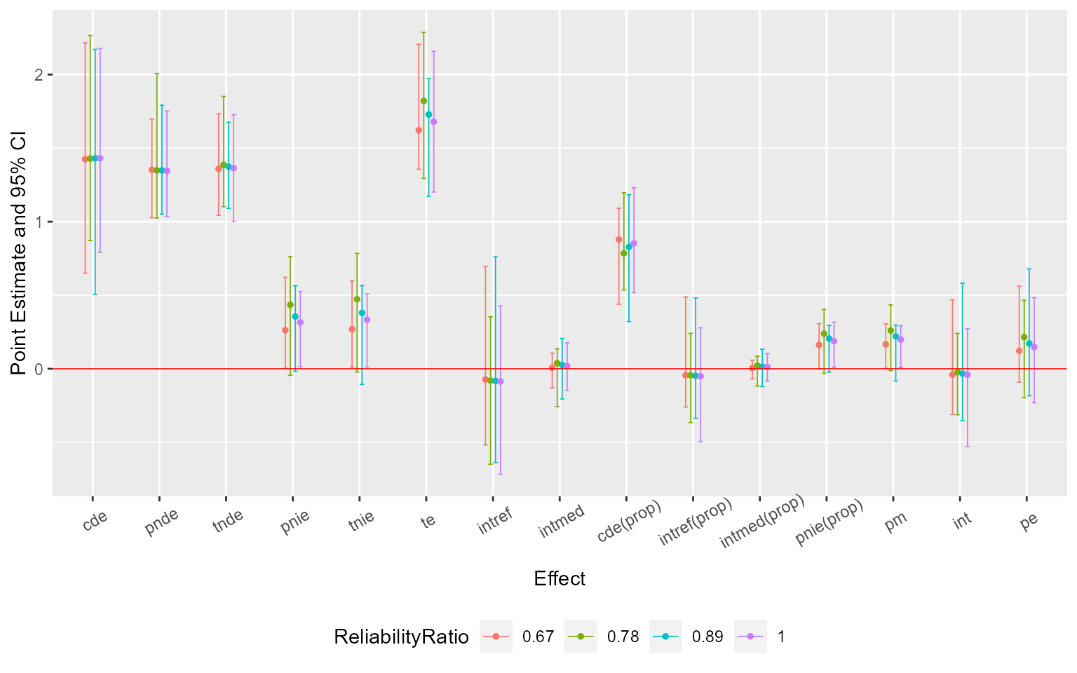
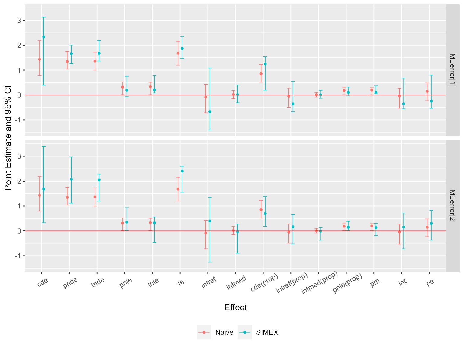
Then, assume that the exposure was measured with error. Sensitivity analysis for measurement error using SIMEX with two assumed misclassification matrices:
me2 <- cmsens(object = est, sens = "me", MEmethod = "simex", MEvariable = "A",
              MEvartype = "cat", B = 5,
              MEerror = list(matrix(c(0.95, 0.05, 0.05, 0.95), nrow = 2),
                             matrix(c(0.9, 0.1, 0.1, 0.9), nrow = 2)))
Summarize and plot the results:
summary(me2)## Sensitivity Analysis For Measurement Error
##
## The variable measured with error: A
## Type of the variable measured with error: categorical
##
## # Measurement error 1:
## [,1] [,2]
## [1,] 0.95 0.05
## [2,] 0.05 0.95
##
## ## Error-corrected regressions for measurement error 1:
##
## ### Outcome regression:
## Call:
## simexreg(reg = getCall(x$sens[[1L]]$reg.output$yreg)$reg, formula = Y ~
## A + M1 + M2 + A * M1 + A * M2 + C1 + C2, data = getCall(x$sens[[1L]]$reg.output$yreg)$data,
## MEvariable = "A", MEvartype = "categorical", MEerror = c(0.95,
## 0.05, 0.05, 0.95), variance = TRUE, lambda = c(0.5, 1, 1.5,
## 2), B = 5, weights = getCall(x$sens[[1L]]$reg.output$yreg)$weights)
##
## Naive coefficient estimates:
## (Intercept) A M1 M2 C1 C2
## -0.429317055 1.305199111 0.762169424 0.691868043 -0.197349688 2.389790272
## A:M1 A:M2
## 0.127853354 -0.001607689
##
## Naive var-cov estimates:
## (Intercept) A M1 M2 C1
## (Intercept) 0.19952129 -0.186177297 -0.071800151 -0.042143887 -0.012473494
## A -0.18617730 0.565227608 0.061763824 0.035566831 0.008550886
## M1 -0.07180015 0.061763824 0.096603550 0.011127995 0.008367323
## M2 -0.04214389 0.035566831 0.011127995 0.017433949 -0.005541985
## C1 -0.01247349 0.008550886 0.008367323 -0.005541985 0.018737581
## C2 0.03202116 -0.002076496 -0.025485517 -0.031937394 0.011413789
## A:M1 0.05250394 -0.194186113 -0.081844376 0.001218548 -0.006350845
## A:M2 0.03868322 -0.102112096 -0.008061219 -0.010381316 -0.000334026
## C2 A:M1 A:M2
## (Intercept) 0.032021156 0.052503937 0.038683218
## A -0.002076496 -0.194186113 -0.102112096
## M1 -0.025485517 -0.081844376 -0.008061219
## M2 -0.031937394 0.001218548 -0.010381316
## C1 0.011413789 -0.006350845 -0.000334026
## C2 0.126311866 -0.027375016 0.006147880
## A:M1 -0.027375016 0.217618968 0.019236723
## A:M2 0.006147880 0.019236723 0.022850334
##
## Variable measured with error:
## A
## Measurement error:
## 0 1
## 0 0.95 0.05
## 1 0.05 0.95
##
## Error-corrected results:
## Estimate Std. Error t value Pr(>|t|)
## (Intercept) -0.3948 0.3482 -1.134 0.2599
## A 1.8740 NA NA NA
## M1 0.4391 0.3052 1.439 0.1536
## M2 0.7125 0.1249 5.705 1.40e-07 ***
## C1 -0.2333 0.1151 -2.026 0.0456 *
## C2 2.3301 0.3604 6.465 4.77e-09 ***
## A:M1 0.5823 0.5425 1.073 0.2859
## A:M2 -0.1226 NA NA NA
## ---
## Signif. codes: 0 '***' 0.001 '**' 0.01 '*' 0.05 '.' 0.1 ' ' 1
##
## ### Mediator regressions:
## Call:
## simexreg(reg = getCall(x$sens[[1L]]$reg.output$mreg[[1L]])$reg,
## formula = M1 ~ A + C1 + C2, data = getCall(x$sens[[1L]]$reg.output$mreg[[1L]])$data,
## MEvariable = "A", MEvartype = "categorical", MEerror = c(0.95,
## 0.05, 0.05, 0.95), variance = TRUE, lambda = c(0.5, 1, 1.5,
## 2), B = 5, weights = getCall(x$sens[[1L]]$reg.output$mreg[[1L]])$weights)
##
## Naive coefficient estimates:
## (Intercept) A C1 C2
## 0.003446339 0.828694328 -0.984453987 0.892199087
##
## Naive var-cov estimates:
## (Intercept) A C1 C2
## (Intercept) 0.30025921 -0.07438249 -0.08381839 -0.17194314
## A -0.07438249 0.20860406 -0.00266003 -0.01458923
## C1 -0.08381839 -0.00266003 0.08577848 -0.01275232
## C2 -0.17194314 -0.01458923 -0.01275232 0.26197192
##
## Variable measured with error:
## A
## Measurement error:
## 0 1
## 0 0.95 0.05
## 1 0.05 0.95
##
## Error-corrected results:
## Estimate Std. Error t value Pr(>|t|)
## (Intercept) 0.1671 0.5520 0.303 0.7628
## A1 0.6279 0.5216 1.204 0.2317
## C1 -0.9362 0.2899 -3.230 0.0017 **
## C2 0.7649 0.5134 1.490 0.1396
## ---
## Signif. codes: 0 '***' 0.001 '**' 0.01 '*' 0.05 '.' 0.1 ' ' 1
##
## Call:
## simexreg(reg = getCall(x$sens[[1L]]$reg.output$mreg[[2L]])$reg,
## formula = M2 ~ A + C1 + C2, data = getCall(x$sens[[1L]]$reg.output$mreg[[2L]])$data,
## MEvariable = "A", MEvartype = "categorical", MEerror = c(0.95,
## 0.05, 0.05, 0.95), variance = TRUE, lambda = c(0.5, 1, 1.5,
## 2), B = 5, weights = getCall(x$sens[[1L]]$reg.output$mreg[[2L]])$weights)
##
## Naive coefficient estimates:
## (Intercept) A C1 C2
## 1.6402566 0.2901364 0.6208107 2.0833115
##
## Naive var-cov estimates:
## (Intercept) A C1 C2
## (Intercept) 0.06573913 -0.018924346 -0.0173562931 -0.0381103530
## A -0.01892435 0.047073002 0.0032931500 -0.0062472874
## C1 -0.01735629 0.003293150 0.0141472682 0.0003964488
## C2 -0.03811035 -0.006247287 0.0003964488 0.0559647177
##
## Variable measured with error:
## A
## Measurement error:
## 0 1
## 0 0.9 0.1
## 1 0.1 0.9
##
## Error-corrected results:
## Estimate Std. Error t value Pr(>|t|)
## (Intercept) 1.5985 0.2803 5.702 1.30e-07 ***
## A 0.3403 0.3206 1.062 0.291
## C1 0.6341 0.1211 5.235 9.71e-07 ***
## C2 2.0890 0.2390 8.741 7.49e-14 ***
## ---
## Signif. codes: 0 '***' 0.001 '**' 0.01 '*' 0.05 '.' 0.1 ' ' 1
##
##
## ## Error-corrected causal effects on the mean difference scale for measurement error 1:
## Estimate Std.error 95% CIL 95% CIU P.val
## cde 2.333749 0.849479 0.392715 3.134 <2e-16 ***
## pnde 1.663306 0.231381 1.264425 2.003 <2e-16 ***
## tnde 1.675689 0.215797 1.364257 2.187 <2e-16 ***
## pnie 0.195664 0.229201 -0.069716 0.751 0.2
## tnie 0.208046 0.198643 0.081955 0.788 <2e-16 ***
## te 1.871352 0.264569 1.473680 2.360 <2e-16 ***
## intref -0.670443 0.732911 -1.404194 1.088 0.8
## intmed 0.012383 0.197096 -0.314801 0.398 0.9
## cde(prop) 1.247092 0.401435 0.198257 1.535 <2e-16 ***
## intref(prop) -0.358267 0.366638 -0.672400 0.549 0.8
## intmed(prop) 0.006617 0.092040 -0.135806 0.189 0.9
## pnie(prop) 0.104557 0.101725 -0.035695 0.322 0.2
## pm 0.111174 0.088811 0.048394 0.365 <2e-16 ***
## int -0.351650 0.381562 -0.557131 0.686 0.8
## pe -0.247092 0.401435 -0.535386 0.802 0.8
## ---
## Signif. codes: 0 '***' 0.001 '**' 0.01 '*' 0.05 '.' 0.1 ' ' 1
## ----------------------------------------------------------------
##
## # Measurement error 2:
## [,1] [,2]
## [1,] 0.9 0.1
## [2,] 0.1 0.9
##
## ## Error-corrected regressions for measurement error 2:
##
## ### Outcome regression:
## Call:
## simexreg(reg = getCall(x$sens[[2L]]$reg.output$yreg)$reg, formula = Y ~
## A + M1 + M2 + A * M1 + A * M2 + C1 + C2, data = getCall(x$sens[[2L]]$reg.output$yreg)$data,
## MEvariable = "A", MEvartype = "categorical", MEerror = c(0.9,
## 0.1, 0.1, 0.9), variance = TRUE, lambda = c(0.5, 1, 1.5,
## 2), B = 5, weights = getCall(x$sens[[2L]]$reg.output$yreg)$weights)
##
## Naive coefficient estimates:
## (Intercept) A M1 M2 C1 C2
## -0.429317055 1.305199111 0.762169424 0.691868043 -0.197349688 2.389790272
## A:M1 A:M2
## 0.127853354 -0.001607689
##
## Naive var-cov estimates:
## (Intercept) A M1 M2 C1
## (Intercept) 0.19952129 -0.186177297 -0.071800151 -0.042143887 -0.012473494
## A -0.18617730 0.565227608 0.061763824 0.035566831 0.008550886
## M1 -0.07180015 0.061763824 0.096603550 0.011127995 0.008367323
## M2 -0.04214389 0.035566831 0.011127995 0.017433949 -0.005541985
## C1 -0.01247349 0.008550886 0.008367323 -0.005541985 0.018737581
## C2 0.03202116 -0.002076496 -0.025485517 -0.031937394 0.011413789
## A:M1 0.05250394 -0.194186113 -0.081844376 0.001218548 -0.006350845
## A:M2 0.03868322 -0.102112096 -0.008061219 -0.010381316 -0.000334026
## C2 A:M1 A:M2
## (Intercept) 0.032021156 0.052503937 0.038683218
## A -0.002076496 -0.194186113 -0.102112096
## M1 -0.025485517 -0.081844376 -0.008061219
## M2 -0.031937394 0.001218548 -0.010381316
## C1 0.011413789 -0.006350845 -0.000334026
## C2 0.126311866 -0.027375016 0.006147880
## A:M1 -0.027375016 0.217618968 0.019236723
## A:M2 0.006147880 0.019236723 0.022850334
##
## Variable measured with error:
## A
## Measurement error:
## 0 1
## 0 0.9 0.1
## 1 0.1 0.9
##
## Error-corrected results:
## Estimate Std. Error t value Pr(>|t|)
## (Intercept) -0.19219 0.33891 -0.567 0.5720
## A 1.77271 0.77710 2.281 0.0248 *
## M1 0.55598 0.41379 1.344 0.1824
## M2 0.51478 0.11915 4.320 3.93e-05 ***
## C1 -0.08903 0.11618 -0.766 0.4455
## C2 2.62126 0.31421 8.342 6.96e-13 ***
## A:M1 -0.19204 0.65071 -0.295 0.7686
## A:M2 0.09880 0.17026 0.580 0.5631
## ---
## Signif. codes: 0 '***' 0.001 '**' 0.01 '*' 0.05 '.' 0.1 ' ' 1
##
## ### Mediator regressions:
## Call:
## simexreg(reg = getCall(x$sens[[2L]]$reg.output$mreg[[1L]])$reg,
## formula = M1 ~ A + C1 + C2, data = getCall(x$sens[[2L]]$reg.output$mreg[[1L]])$data,
## MEvariable = "A", MEvartype = "categorical", MEerror = c(0.9,
## 0.1, 0.1, 0.9), variance = TRUE, lambda = c(0.5, 1, 1.5,
## 2), B = 5, weights = getCall(x$sens[[2L]]$reg.output$mreg[[1L]])$weights)
##
## Naive coefficient estimates:
## (Intercept) A C1 C2
## 0.003446339 0.828694328 -0.984453987 0.892199087
##
## Naive var-cov estimates:
## (Intercept) A C1 C2
## (Intercept) 0.30025921 -0.07438249 -0.08381839 -0.17194314
## A -0.07438249 0.20860406 -0.00266003 -0.01458923
## C1 -0.08381839 -0.00266003 0.08577848 -0.01275232
## C2 -0.17194314 -0.01458923 -0.01275232 0.26197192
##
## Variable measured with error:
## A
## Measurement error:
## 0 1
## 0 0.95 0.05
## 1 0.05 0.95
##
## Error-corrected results:
## Estimate Std. Error t value Pr(>|t|)
## (Intercept) 0.1671 0.5520 0.303 0.7628
## A1 0.6279 0.5216 1.204 0.2317
## C1 -0.9362 0.2899 -3.230 0.0017 **
## C2 0.7649 0.5134 1.490 0.1396
## ---
## Signif. codes: 0 '***' 0.001 '**' 0.01 '*' 0.05 '.' 0.1 ' ' 1
##
## Call:
## simexreg(reg = getCall(x$sens[[2L]]$reg.output$mreg[[2L]])$reg,
## formula = M2 ~ A + C1 + C2, data = getCall(x$sens[[2L]]$reg.output$mreg[[2L]])$data,
## MEvariable = "A", MEvartype = "categorical", MEerror = c(0.9,
## 0.1, 0.1, 0.9), variance = TRUE, lambda = c(0.5, 1, 1.5,
## 2), B = 5, weights = getCall(x$sens[[2L]]$reg.output$mreg[[2L]])$weights)
##
## Naive coefficient estimates:
## (Intercept) A C1 C2
## 1.6402566 0.2901364 0.6208107 2.0833115
##
## Naive var-cov estimates:
## (Intercept) A C1 C2
## (Intercept) 0.06573913 -0.018924346 -0.0173562931 -0.0381103530
## A -0.01892435 0.047073002 0.0032931500 -0.0062472874
## C1 -0.01735629 0.003293150 0.0141472682 0.0003964488
## C2 -0.03811035 -0.006247287 0.0003964488 0.0559647177
##
## Variable measured with error:
## A
## Measurement error:
## 0 1
## 0 0.9 0.1
## 1 0.1 0.9
##
## Error-corrected results:
## Estimate Std. Error t value Pr(>|t|)
## (Intercept) 1.5985 0.2803 5.702 1.30e-07 ***
## A 0.3403 0.3206 1.062 0.291
## C1 0.6341 0.1211 5.235 9.71e-07 ***
## C2 2.0890 0.2390 8.741 7.49e-14 ***
## ---
## Signif. codes: 0 '***' 0.001 '**' 0.01 '*' 0.05 '.' 0.1 ' ' 1
##
##
## ## Error-corrected causal effects on the mean difference scale for measurement error 2:
## Estimate Std.error 95% CIL 95% CIU P.val
## cde 1.67947 1.08720 0.32807 3.399 <2e-16 ***
## pnde 2.07886 0.49879 1.11599 2.970 <2e-16 ***
## tnde 2.05103 0.31573 1.19583 2.285 <2e-16 ***
## pnie 0.35310 0.25901 0.01610 0.934 0.1 .
## tnie 0.32527 0.30363 -0.45864 0.565 0.2
## te 2.40413 0.32522 1.55424 2.596 <2e-16 ***
## intref 0.39939 0.77596 -1.24944 1.353 0.7
## intmed -0.02783 0.34260 -0.89762 0.274 0.9
## cde(prop) 0.69858 0.42020 0.18019 1.376 <2e-16 ***
## intref(prop) 0.16613 0.37337 -0.52542 0.653 0.7
## intmed(prop) -0.01158 0.14877 -0.37550 0.135 0.9
## pnie(prop) 0.14687 0.10723 0.01021 0.384 0.1 .
## pm 0.13530 0.14201 -0.18833 0.303 0.2
## int 0.15455 0.47312 -0.71832 0.719 0.9
## pe 0.30142 0.42020 -0.37555 0.820 0.7
## ---
## Signif. codes: 0 '***' 0.001 '**' 0.01 '*' 0.05 '.' 0.1 ' ' 1
## ----------------------------------------------------------------
##
## (cde: controlled direct effect; pnde: pure natural direct effect; tnde: total natural direct effect; pnie: pure natural indirect effect; tnie: total natural indirect effect; te: total effect; intref: reference interaction; intmed: mediated interaction; cde(prop): proportion cde; intref(prop): proportion intref; intmed(prop): proportion intmed; pnie(prop): proportion pnie; pm: overall proportion mediated; int: overall proportion attributable to interaction; pe: overall proportion eliminated)
##
## Relevant variable values:
## $a
## [1] 1
##
## $astar
## [1] 0
##
## $mval
## $mval[[1]]
## [1] 1
##
## $mval[[2]]
## [1] 1
ggcmsens(me2) +
  ggplot2::theme(axis.text.x = ggplot2::element_text(angle = 30, vjust = 0.8))